use https://stats.idre.ucla.edu/stat/stata/examples/chp/p203, clear

generate index = _n
Table 8.1, page 203.
Note: Create the variable index equal to the observation number.
list

         year   quarter   expendit      stock      index
  1.     1952         1      214.6      159.3          1
  2.     1952         2      217.7      161.2          2
  3.     1952         3      219.6      162.8          3
  4.     1952         4      227.2      164.6          4
  5.     1953         1      230.9      165.9          5
  6.     1953         2      233.3      167.9          6
  7.     1953         3      234.1      168.3          7
  8.     1953         4      232.3      169.7          8
  9.     1954         1      233.7      170.5          9
 10.     1954         2      236.5      171.6         10
 11.     1954         3      238.7      173.9         11
 12.     1954         4      243.2      176.1         12
 13.     1955         1      249.4        178         13
 14.     1955         2      254.3      179.1         14
 15.     1955         3      260.9      180.2         15
 16.     1955         4      263.3      181.2         16
 17.     1956         1      265.6      181.6         17
 18.     1956         2      268.2      182.5         18
 19.     1956         3      270.4      183.3         19
 20.     1956         4      275.6      184.3         20
Table 8.2, page 203.
regress expendit stock

  Source |       SS       df       MS                  Number of obs =      20
---------+------------------------------               F(  1,    18) =  403.22
   Model |  6395.76619     1  6395.76619               Prob > F      =  0.0000
Residual |  285.511158    18   15.861731               R-squared     =  0.9573
---------+------------------------------               Adj R-squared =  0.9549
   Total |  6681.27735    19  351.646176               Root MSE      =  3.9827

------------------------------------------------------------------------------
expendit |      Coef.   Std. Err.       t     P>|t|       [95% Conf. Interval]
---------+--------------------------------------------------------------------
   stock |    2.30037   .1145584     20.080   0.000       2.059692    2.541049
   _cons |  -154.7191   19.85004     -7.794   0.000      -196.4225   -113.0157
------------------------------------------------------------------------------
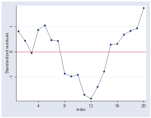
Figure 8.1, page 204.
Note: The connect(l) option is used to connect the plotted points with a line.
predict r, rstandard
graph twoway scatter r index, c(l) ylabel(-1 0 1) xlabel(4(4)20) yline(0)
Durbin-Watson statistic, page 205.
tsset index

*Stata 8 code.
dwstat

* Stata 9 code and output.
estat dwatson

Durbin-Watson d-statistic(  2,    20) =  .3282105
Equation at the bottom of page 207.
Note: The prais command is used to perform Cochrane-Orcutt transformation. The
two option stops the procedure after the first estimate of rho.
prais expendit stock, corc two rhotype(tsc)

Iteration 0:  rho = 0.0000
Iteration 1:  rho = 0.7506

Cochrane-Orcutt AR(1) regression -- twostep estimates

  Source |       SS       df       MS                  Number of obs =      19
---------+------------------------------               F(  1,    17) =   74.20
   Model |  379.837381     1  379.837381               Prob > F      =  0.0000
Residual |  87.0261726    17  5.11918663               R-squared     =  0.8136
---------+------------------------------               Adj R-squared =  0.8026
   Total |  466.863554    18  25.9368641               Root MSE      =  2.2626

------------------------------------------------------------------------------
expendit |      Coef.   Std. Err.       t     P>|t|       [95% Conf. Interval]
---------+--------------------------------------------------------------------
   stock |   2.643445   .3068823      8.614   0.000        1.99598     3.29091
   _cons |  -215.3112   54.59925     -3.943   0.001      -330.5056   -100.1169
------------------------------------------------------------------------------
     rho |   .7506127
------------------------------------------------------------------------------
Durbin-Watson statistic (original)    0.328210
Durbin-Watson statistic (transformed) 1.425962
Iterative solution; Table 8.1, page 209.
prais expendit stock, corc

Iteration 0:  rho = 0.0000
Iteration 1:  rho = 0.8745
Iteration 2:  rho = 0.8422
Iteration 3:  rho = 0.8295
Iteration 4:  rho = 0.8255
Iteration 5:  rho = 0.8244
Iteration 6:  rho = 0.8242
Iteration 7:  rho = 0.8241
Iteration 8:  rho = 0.8241
Iteration 9:  rho = 0.8241
Iteration 10:  rho = 0.8241
Iteration 11:  rho = 0.8241

Cochrane-Orcutt AR(1) regression -- iterated estimates

  Source |       SS       df       MS                  Number of obs =      19
---------+------------------------------               F(  1,    17) =   39.79
   Model |  198.494803     1  198.494803               Prob > F      =  0.0000
Residual |  84.8128884    17  4.98899343               R-squared     =  0.7006
---------+------------------------------               Adj R-squared =  0.6830
   Total |  283.307691    18  15.7393162               Root MSE      =  2.2336

------------------------------------------------------------------------------
expendit |      Coef.   Std. Err.       t     P>|t|       [95% Conf. Interval]
---------+--------------------------------------------------------------------
   stock |    2.75306   .4364632      6.308   0.000       1.832204    3.673917
   _cons |  -235.4889   78.61251     -2.996   0.008      -401.3468     -69.631
------------------------------------------------------------------------------
     rho |   .8240543
------------------------------------------------------------------------------
Durbin-Watson statistic (original)    0.328210
Durbin-Watson statistic (transformed) 1.601029
Table 8.4, page 211.
use https://stats.idre.ucla.edu/stat/stata/examples/chp/p211, clear
generate index = _n
list

             h          p          d      index
  1.     .0909        2.2     .03635          1
  2.    .08942      2.222     .03345          2
  3.    .09755      2.244      .0387          3
  4.     .0955      2.267     .03745          4
  5.    .09678       2.28     .04063          5
  6.    .10327      2.289     .04237          6
  7.    .10513      2.289     .04715          7
  8.     .1084       2.29     .04883          8
  9.    .10822      2.299     .04836          9
 10.    .10741        2.3      .0516         10
 11.    .10751        2.3     .04879         11
 12.    .11429       2.34     .05523         12
 13.    .11048      2.386      .0477         13
 14.    .11604      2.433     .05282         14
 15.    .11688      2.482     .05473         15
 16.    .12044      2.532     .05531         16
 17.    .12125       2.58     .05898         17
 18.     .1208      2.605     .06267         18
 19.    .12368      2.631     .05462         19
 20.    .12679      2.658     .05672         20
 21.    .12996      2.684     .06674         21
 22.    .13445      2.711     .06451         22
 23.    .13325      2.738     .06313         23
 24.    .13863      2.766     .06573         24
 25.    .13964      2.793     .07229         25
Table 8.5, page 212.
regress h p

  Source |       SS       df       MS                  Number of obs =      25
---------+------------------------------               F(  1,    23) =  284.51
   Model |  .004736628     1  .004736628               Prob > F      =  0.0000
Residual |  .000382913    23  .000016648               R-squared     =  0.9252
---------+------------------------------               Adj R-squared =  0.9220
   Total |  .005119541    24  .000213314               Root MSE      =  .00408

------------------------------------------------------------------------------
       h |      Coef.   Std. Err.       t     P>|t|       [95% Conf. Interval]
---------+--------------------------------------------------------------------
       p |   .0714097   .0042336     16.867   0.000       .0626518    .0801675
   _cons |   -.060884    .010416     -5.845   0.000      -.0824311   -.0393369
------------------------------------------------------------------------------
Figure 8.3, page 212.
predict r1, rstandard
graph twoway scatter r1 index, c(l) ylabel(-2(1)1) xlabel(5(5)25) yline(0)
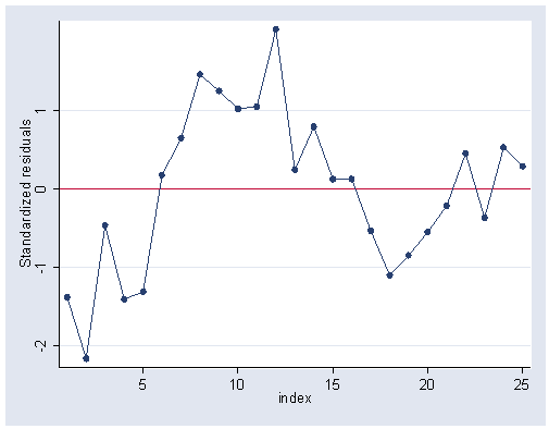
Table 8.6, page 213.
regress h p d

  Source |       SS       df       MS                  Number of obs =      25
---------+------------------------------               F(  2,    22) =  397.58
   Model |  .004981709     2  .002490854               Prob > F      =  0.0000
Residual |  .000137833    22  6.2651e-06               R-squared     =  0.9731
---------+------------------------------               Adj R-squared =  0.9706
   Total |  .005119541    24  .000213314               Root MSE      =   .0025

------------------------------------------------------------------------------
       h |      Coef.   Std. Err.       t     P>|t|       [95% Conf. Interval]
---------+--------------------------------------------------------------------
       p |   .0346557   .0064248      5.394   0.000       .0213315    .0479798
       d |   .7604638   .1215875      6.254   0.000       .5083067    1.012621
   _cons |  -.0104272   .0102913     -1.013   0.322      -.0317699    .0109156
------------------------------------------------------------------------------
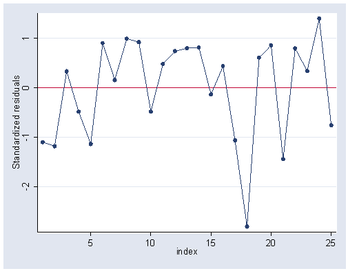
Figure 8.4, page 213.
predict r2, rstandard
graph twoway scatter r2 index, c(l) ylabel(-2(1)1) xlabel(5(5)25) yline(0)
Equation top of page 214.
regress h p d, beta

  Source |       SS       df       MS                  Number of obs =      25
---------+------------------------------               F(  2,    22) =  397.58
   Model |  .004981709     2  .002490854               Prob > F      =  0.0000
Residual |  .000137833    22  6.2651e-06               R-squared     =  0.9731
---------+------------------------------               Adj R-squared =  0.9706
   Total |  .005119541    24  .000213314               Root MSE      =   .0025

------------------------------------------------------------------------------
       h |      Coef.   Std. Err.       t     P>|t|                       Beta
---------+--------------------------------------------------------------------
       p |   .0346557   .0064248      5.394   0.000                   .4668058
       d |   .7604638   .1215875      6.254   0.000                   .5412634
   _cons |  -.0104272   .0102913     -1.013   0.322                          .
------------------------------------------------------------------------------
use https://stats.idre.ucla.edu/stat/stata/examples/chp/p217, clear
generate index = _n
Table 8.7, page 215.
regress sales pdi

  Source |       SS       df       MS                  Number of obs =      40
---------+------------------------------               F(  1,    38) =  152.55
   Model |  1390.73632     1  1390.73632               Prob > F      =  0.0000
Residual |  346.433325    38  9.11666646               R-squared     =  0.8006
---------+------------------------------               Adj R-squared =  0.7953
   Total |  1737.16965    39  44.5428115               Root MSE      =  3.0194

------------------------------------------------------------------------------
   sales |      Coef.   Std. Err.       t     P>|t|       [95% Conf. Interval]
---------+--------------------------------------------------------------------
     pdi |   .1979142   .0160241     12.351   0.000       .1654752    .2303533
   _cons |   12.39215   2.539425      4.880   0.000       7.251353    17.53295
------------------------------------------------------------------------------
Figure 8.5, page 215.
predict r3, rstandard
graph twoway (scatter r3 index if season == 1, msymbol(X) yvarlabel("Q1 & Q4")) ///
	(scatter r3 index if season == 0, msymbol(Oh) yvarlabel("Q2 & Q3")), ///
	ylabel(-1.5(.75)1.5)
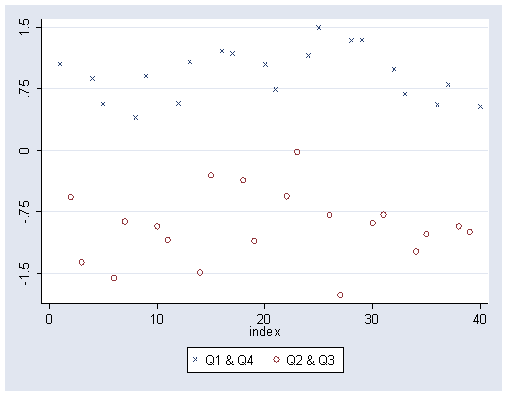
Table 8.8, page 217.
list

       quarter      sales       pdi    season      index
  1.     Q1/64         37       109         1          1
  2.     Q2/64       33.5       115         0          2
  3.     Q3/64       30.8       113         0          3
  4.     Q4/64       37.9       116         1          4
  5.     Q1/65       37.4       118         1          5
  6.     Q2/65       31.6       120         0          6
  7.     Q3/65         34       122         0          7
  8.     Q4/65       38.1       124         1          8
  9.     Q1/66         40       126         1          9
 10.     Q2/66         35       128         0         10
..
 [remainder of output omitted]
Table 8.9, page 217.
regress sales pdi season

  Source |       SS       df       MS                  Number of obs =      40
---------+------------------------------               F(  2,    37) =  652.94
   Model |  1689.30565     2  844.652823               Prob > F      =  0.0000
Residual |  47.8640016    37  1.29362167               R-squared     =  0.9724
---------+------------------------------               Adj R-squared =  0.9710
   Total |  1737.16965    39  44.5428115               Root MSE      =  1.1374

------------------------------------------------------------------------------
   sales |      Coef.   Std. Err.       t     P>|t|       [95% Conf. Interval]
---------+--------------------------------------------------------------------
     pdi |   .1986837   .0060363     32.915   0.000        .186453    .2109145
  season |   5.464342   .3596822     15.192   0.000       4.735557    6.193127
   _cons |   9.540204   .9748254      9.787   0.000        7.56502    11.51539
------------------------------------------------------------------------------
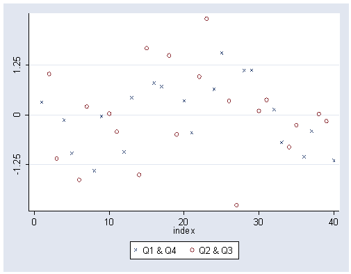
Figure 8.7, page 218.
predict r4, rstandard
graph twoway (scatter r4 index if season == 1, msymbol(X) yvarlabel("Q1 & Q4")) ///
	(scatter r4 index if season == 0, msymbol(Oh) yvarlabel("Q2 & Q3")), ///
	ylabel(-1.25 0 1.25)