/* Table 7.3, page 189. */

use https://stats.idre.ucla.edu/stat/stata/examples/chp/p189, clear

list


         state         y        x1        x2        x3    region
  1.        ME       235      3944       325       508         1
  2.        NH       231      4578       323       564         1
  3.        VT       270      4011       328       322         1
  4.        MA       261      5233       305       846         1
  5.        RI       300      4780       303       871         1
  6.        CT       317      5889       307       774         1
  7.        NY       387      5663       301       856         1
  8.        NJ       285      5759       310       889         1
  9.        PA       300      4894       300       715         1
 10.        OH       221      5012       324       753         2
..
 [remainder of output deleted]


/* Table 7.4, page 191 */

regress y x1 x2 x3


  Source |       SS       df       MS                  Number of obs =      50
---------+------------------------------               F(  3,    46) =   22.19
   Model |  109020.418     3  36340.1394               Prob > F      =  0.0000
Residual |  75347.5819    46  1637.99091               R-squared     =  0.5913
---------+------------------------------               Adj R-squared =  0.5647
   Total |   184368.00    49  3762.61224               Root MSE      =  40.472

------------------------------------------------------------------------------
       y |      Coef.   Std. Err.       t     P>|t|       [95% Conf. Interval]
---------+--------------------------------------------------------------------
      x1 |   .0723853   .0116024      6.239   0.000       .0490308    .0957398
      x2 |   1.552054   .3146716      4.932   0.000       .9186534    2.185456
      x3 |   -.004269   .0513929     -0.083   0.934      -.1077175    .0991794
   _cons |   -556.568   123.1953     -4.518   0.000      -804.5472   -308.5889
------------------------------------------------------------------------------


/* Figure 7.3, page 191. */

/* In the book the outlying data point is AL, in our data set that
   point corresponds to AK. */

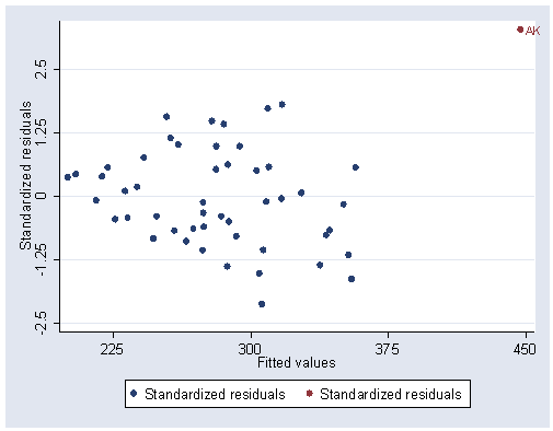
predict p
predict r, rstandard

graph twoway (scatter r p) (scatter r p if state == "AK", mlabel(state)), ///
		ylabel(-2.5(1.25)2.5) xlabel(225(75)450)
/* Figure 7.4, page 191 */

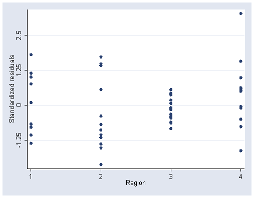
graph twoway scatter r region, ylabel(-1.25(1.25)2.5) xlabel(1(1)4)
/* Figure 7.5, page 192 */

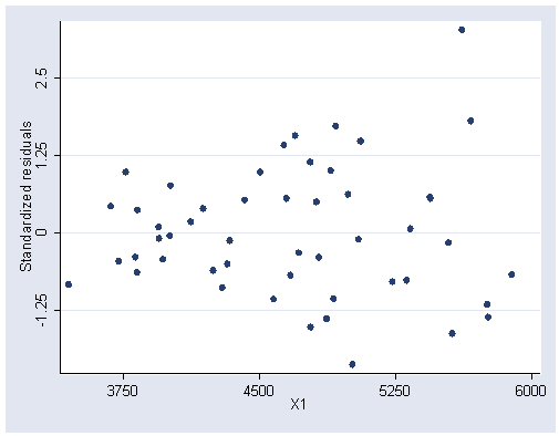
graph twoway scatter r x1, ylabel(-1.25(1.25)2.5)
xlabel(3750(750)6000)
/* Figure 7.6, page 192 */

graph twoway scatter r x2, ylabel(-1.25(1.25)2.5) xlabel(300(25)375)
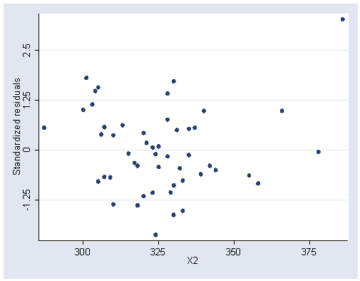
/* Figure 7.7, page 192 */

graph twoway scatter r x3, ylabel(-1.25(1.25)2.5) xlabel(450(150)900)
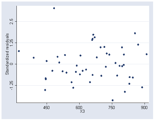
/* Table 7.5, page 193 */

drop if state=="AK"
regress y x1 x2 x3


  Source |       SS       df       MS                  Number of obs =      49
---------+------------------------------               F(  3,    45) =   14.80
   Model |  56943.7919     3   18981.264               Prob > F      =  0.0000
Residual |  57699.7591    45  1282.21687               R-squared     =  0.4967
---------+------------------------------               Adj R-squared =  0.4631
   Total |  114643.551    48  2388.40731               Root MSE      =  35.808

------------------------------------------------------------------------------
       y |      Coef.   Std. Err.       t     P>|t|       [95% Conf. Interval]
---------+--------------------------------------------------------------------
      x1 |   .0482933    .012147      3.976   0.000       .0238281    .0727586
      x2 |   .8869283     .33114      2.678   0.010        .219978    1.553879
      x3 |   .0667917     .04934      1.354   0.183      -.0325841    .1661675
   _cons |  -277.5773   132.4229     -2.096   0.042      -544.2906   -10.86399
------------------------------------------------------------------------------


/* Figure 7.8, page 194 */

predict p2
predict r2, rstandard
graph twoway scatter r2 p2, ylabel(-1.25 0 1.25) xlabel(240 280 320)
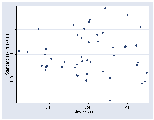
/* Figure 7.9, page 194 */

graph twoway scatter r2 region, ylabel(-2.5(1.25)2.5) xlabel(1(1)4)
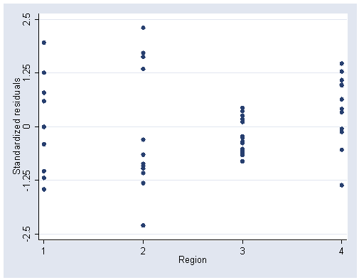
/* Part of Table 7.6, page 195 */

/* Computing the weights from the data */

regress y x1 x2 x3
predict e, resid
generate e2 = e^2
bysort region: gen count = _N
gen e2_adj = e2/(count-1)
egen s2 = sum(e2_adj), by(region)
summarize e2

    Variable |       Obs        Mean    Std. Dev.       Min        Max
-------------+--------------------------------------------------------
          e2 |        49    1177.546    1529.095   .0054078   6581.732


generate c = sqrt(s2/r(mean))
table region, contents(freq mean c)

----------------------------------
   Region |      Freq.     mean(c)
----------+-----------------------
        1 |          9    1.177438
        2 |         12    1.502558
        3 |         16     .475338
        4 |         12    .9383478
----------------------------------


/* Part of Table 7.7, page 195 */

regress y x1 x2 x3 [aw=1/c^2]

(sum of wgt is   9.6249e+01)

      Source |       SS       df       MS              Number of obs =      49
-------------+------------------------------           F(  3,    45) =   47.62
       Model |  76012.6369     3  25337.5456           Prob > F      =  0.0000
    Residual |  23943.4288    45  532.076197           R-squared     =  0.7605
-------------+------------------------------           Adj R-squared =  0.7445
       Total |  99956.0657    48  2082.41804           Root MSE      =  23.067

------------------------------------------------------------------------------
           y |      Coef.   Std. Err.      t    P>|t|     [95% Conf. Interval]
-------------+----------------------------------------------------------------
          x1 |   .0624611   .0078028     8.00   0.000     .0467455    .0781767
          x2 |   .8739911   .1983961     4.41   0.000     .4744008    1.273581
          x3 |   .0289241   .0339939     0.85   0.399    -.0395432    .0973914
       _cons |  -316.0237   77.41892    -4.08   0.000    -471.9535    -160.094
------------------------------------------------------------------------------


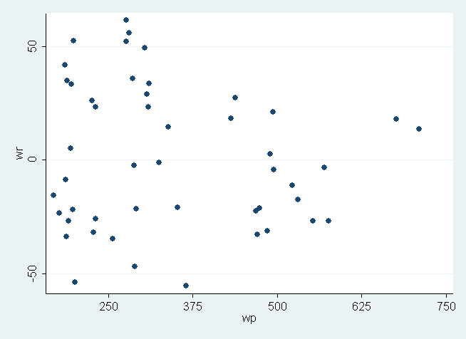
/* Figure 7.10, page 196 */
/* Note 1: Predicted values and residuals need to be adjusted for by the weights used in the wls.*/
/* Note 2: For this figure and the next, Stata does not compute standardized residuals for
weighted data, therefore we are going to use the unstandardized residuals.*/

predict p3
predict r3, residual
generate wp = p3*1/c
generate wr = r3*1/c
graph twoway scatter wr wp, xlabel(250(125)750)
/* Figure 7.11, page 196 */
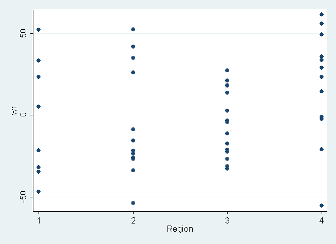
graph twoway scatter wr region, xlabel(1(1)4)