NOTE: Before we being working with the data, we rename the variables to match those used in the text and add variable labels to gender and job. Also note that the variable GPA does not appear in the data set the way the it appears in the graphs in this chapter. Therefore, we have not included the graphs that involve the variable GPA.
use "a:classsur.dta", clear
rename col1 gender
rename col2 age
rename col3 gpa
rename col4 class
rename col5 height
rename col6 weight
rename col7 studyhr
rename col8 sleephr
rename col9 job
rename col10 textpay
rename col11  reside
destring gpa height weight studyhr, replace
label define gend 1 "male" 2 "female"
label values gender gend
label define job1 1 "have job" 2 "don't have job"
label values job job1
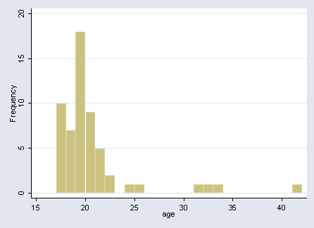
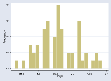
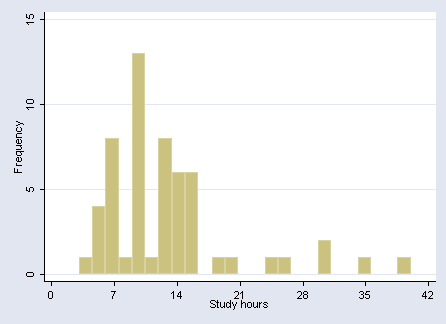
Page 9, Figure 2.1 We use the bin(#) option to tell Stata how many bins to include in the histogram.
histogram age, freq xlabel(15 20 to 40) bin(25)
histogram height, freq xlabel(59.5(3.5)77) xtitle("Height") bin(25)
histogram studyhr, freq xlabel(0(7)42) xtitle("Study hours") bin(25)
Page 11, Figure 2.2
stem age
Stem-and-leaf plot for age

  1s | 7777
  1. | 8888889999999
  2* | 000000000000000000111111111
  2t | 2222233
  2f | 5
  2s | 6
  2. |
  3* |
  3t | 23
  3f | 4
  3s |
  3. |
  4* |
  4t | 2
stem height
Stem-and-leaf plot for height

  5. | 8
  6* | 0111
  6t | 22333
  6f | 44444555555
  6s | 666677777777
  6. | 8888899
  7* | 00111111
  7t | 233
  7f | 455
  7s | 6
stem studyhr
Stem-and-leaf plot for studyhr

  0* | 3
  0. | 5555667777778999
  1* | 0000000000122223333444444
  1. | 5555668
  2* | 0
  2. | 56
  3* | 00
  3. | 5
  4* | 0
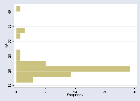
Page 12, Figure 2.3 We use the option horizontal (abbreviated hor) to make the histogram horizontal. Note the when making graphs horizontal, Stata rotates the axes. Hence, you need to use the ytitle option (instead of the xtitle) to put a label on the bottom axis. We also use the start(#) option to tell Stata what value with which to start the lowest bin.
histogram age, bin(14) freq xlabel(0(7)28) hor start(16)
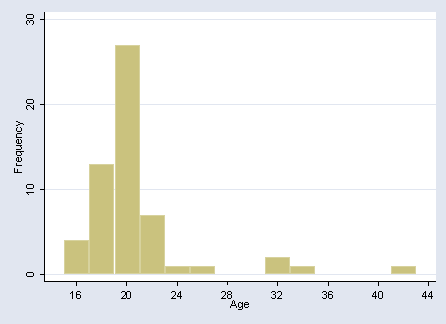
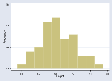
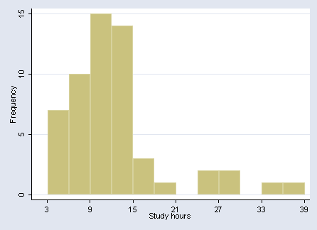
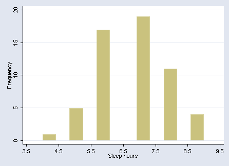
Page 13, Figure 2.4 We use the width(#) option to tell Stata how wide to make each bin. Note that you can not use both the bin(#) and the width(#) option for the same histogram.
histogram age, width(2) freq xlabel(16(4)44) xtitle("Age") ylabel(0(10)30) start(15)
histogram height, width(2) freq xlabel(58(4)78) xtitle("Height") ylabel(0(5)15) start(57)
histogram studyhr, width(3) freq xlabel(3(6)39) ylabel(0(5)15) xtitle("Study hours") start(3)
histogram sleephr, freq xlabel(3.5(1)9.5) xtitle("Sleep hours") bin(12)
NOTE: We were unable to make this graph look more like the one in the text.
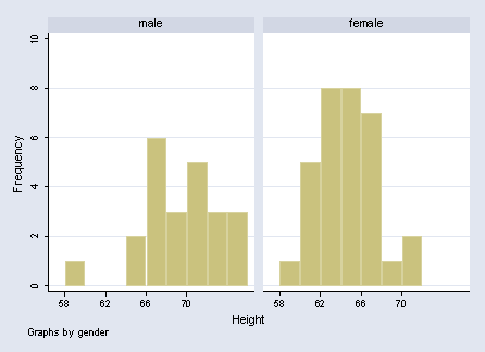
Page 14, Figure 2.5 NOTE: The graphs below are in the reverse order of those shown in the text.
histogram height, by(gender) freq width(2) xlabel(58(4)70) xtitle("Height") ylabel(0(2)10)
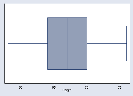
Page 15, Figure 2.6 We use hbox to make the boxplot horizontal. Note the when making graphs horizontal, Stata rotates the axes. Hence, you need to use the ytitle option (instead of the xtitle) to put a label on the bottom axis.
graph hbox height, ytitle("Height") ylabel(60(5)75)
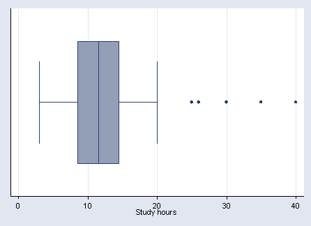
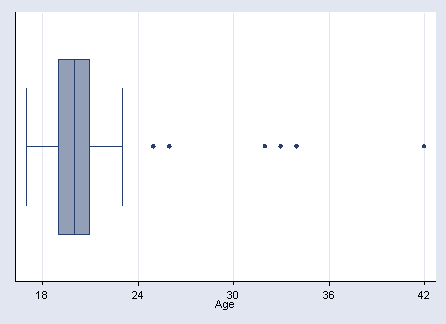
Page 16, Figure 2.7
graph hbox studyhr, ytitle("Study hours") ylabel(0(10)40)
graph hbox age, ytitle("Age") ylabel(18(6)42)
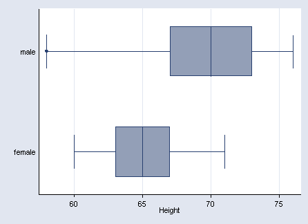
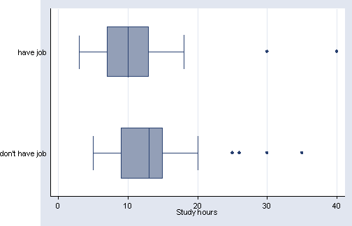
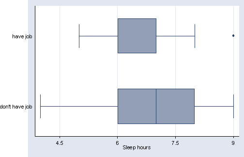
Page 17, Figure 2.8 We use over() to get the boxplots one above the other, instead of side-by-side as by() would produce.
graph hbox height, over(gender) ytitle("Height") ylabel(60(5)75)
graph hbox studyhr, over(job) ytitle("Study hours") ylabel(0(10)40)
graph hbox sleephr, over(job) ytitle("Sleep hours") ylabel(4.5(1.5)9)
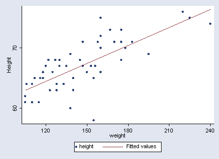
Page 2.9, Figure 2.9 We use the three slashes (///) at the end of the line to tell Stata to ignore the return and continue reading the current command on the next line. This is feature that is new to Stata 8 and can be used instead of the /* */ that used to contain the return.
twoway (scatter height weight) (lfit height weight), ///
ytitle("Height") xlabel(120(30)240) ylabel(60 70, nogrid)
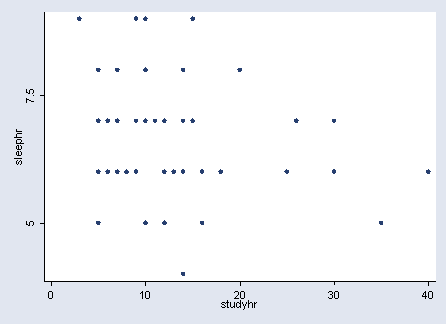
Page 19, Figure 2.11 We use the nogrid option in the ylabel option to remove the grid lines that are shown by default.
twoway (scatter sleephr studyhr), xlabel(0(10)40) ylabel(5 7.5, nogrid)
Page 20, Table 2.1
tab job
           job |      Freq.     Percent        Cum.
---------------+-----------------------------------
      have job |         26       45.61       45.61
don't have job |         31       54.39      100.00
---------------+-----------------------------------
         Total |         57      100.00
Page 20, Table 2.2
tab sleephr
    sleephr |      Freq.     Percent        Cum.
------------+-----------------------------------
          4 |          1        1.75        1.75
          5 |          5        8.77       10.53
          6 |         17       29.82       40.35
          7 |         19       33.33       73.68
          8 |         11       19.30       92.98
          9 |          4        7.02      100.00
------------+-----------------------------------
      Total |         57      100.00
Page 2.3, Table 2.3
tab2 gender job
           |          job
    gender |  have job  don't have|     Total
-----------+----------------------+----------
      male |        13         10 |        23
    female |        13         21 |        34
-----------+----------------------+----------
     Total |        26         31 |        57

