NOTE: If you want to see the design effect or the misspecification
effect, use estat effects after the command.
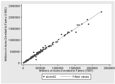
Page 64, figure 3.1
use https://stats.idre.ucla.edu/stat/stata/examples/lohr/agsrs.dta, clear
twoway (scatter acres92 acres87) (lfit acres92 acres87), ylabel( , nogrid angle(0)) ///
  xtitle("Millions of Acres Devoted to Farms (1987)") ///
  ytitle("Millions of Acres Devoted to Farms (1992)")
Page 65, table 3.1
di 297897.0467/301953.7233
gen residual = acres92 - .98656524*acres87
list county state acres92 acres87 residual in 1/6

     +-----------------------------------------------------------+
     |            county   state   acres92   acres87    residual |
     |-----------------------------------------------------------|
  1. |     COFFEE COUNTY      AL    175209    179311       -1693 |
  2. |    COLBERT COUNTY      AL    138135    145104   -5019.563 |
  3. |      LAMAR COUNTY      AL     56102     59861   -2954.782 |
  4. |    MARENGO COUNTY      AL    199117    220526   -18446.29 |
  5. |     MARION COUNTY      AL     89228    105586   -14939.48 |
     |-----------------------------------------------------------|
  6. | TUSCALOOSA COUNTY      AL     96194    120542   -22728.55 |
     +-----------------------------------------------------------+

list county state acres92 acres87  residual in -5/l

     +----------------------------------------------------------+
     |           county   state   acres92   acres87    residual |
     |----------------------------------------------------------|
296. |   OZAUKEE COUNTY      WI     78772     85201   -5284.345 |
297. |      ROCK COUNTY      WI    343115    357751   -9829.701 |
298. |   KANAWHA COUNTY      WV     19956     21369   -1125.913 |
299. | PLEASANTS COUNTY      WV     15650     15716    145.1407 |
300. |    PUTNAM COUNTY      WV     55827     55635    939.4429 |
     +----------------------------------------------------------+

tabstat acres92 acres87 residual, s(sum mean sd) format(%11.0g)

   stats |   acres92   acres87  residual
---------+------------------------------
     sum |   89369114   90586117-.244007111
    mean | 297897.047 301953.723-.000813357
      sd | 344551.895 344829.596 31657.2178
----------------------------------------
Page 72, table 3.3
clear
input tree x y
1 1 0
2 0 0
3 8 1
4 2 2
5 76 10
6 60 15
7 25 3
8 2 2
9 1 1
10 31 27
end

list

     +----------------+
     | tree    x    y |
     |----------------|
  1. |    1    1    0 |
  2. |    2    0    0 |
  3. |    3    8    1 |
  4. |    4    2    2 |
  5. |    5   76   10 |
     |----------------|
  6. |    6   60   15 |
  7. |    7   25    3 |
  8. |    8    2    2 |
  9. |    9    1    1 |
 10. |   10   31   27 |
     +----------------+

tabstat x y, s(sum mean sd)

   stats |         x         y
---------+--------------------
     sum |       206        61
    mean |      20.6       6.1
      sd |  27.47201  8.824839
------------------------------
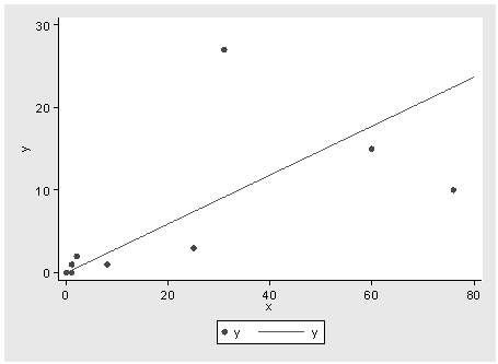
Page 73, figure 3.4
graph twoway (scatter y x) (function y = .2961*x, range(0 80)), ylabel( , nogrid angle(0))
Page 73 in the middle
di 6.1/20.6
.2961165
Page 75 in the middle
clear
input photo field
10 15
12 14
7 9
13 14
13 8
6 5
17 18
16 15
15 13
10 15
14 11
12 15
10 12
5 8
12 13
10 9
10 11
9 12
6 9
11 12
7 13
9 11
11 10
10 9
10 8
end

list

     +---------------+
     | photo   field |
     |---------------|
  1. |    10      15 |
  2. |    12      14 |
  3. |     7       9 |
  4. |    13      14 |
  5. |    13       8 |
     |---------------|
  6. |     6       5 |
  7. |    17      18 |
  8. |    16      15 |
  9. |    15      13 |
 10. |    10      15 |
     |---------------|
 11. |    14      11 |
 12. |    12      15 |
 13. |    10      12 |
 14. |     5       8 |
 15. |    12      13 |
     |---------------|
 16. |    10       9 |
 17. |    10      11 |
 18. |     9      12 |
 19. |     6       9 |
 20. |    11      12 |
     |---------------|
 21. |     7      13 |
 22. |     9      11 |
 23. |    11      10 |
 24. |    10       9 |
 25. |    10       8 |
     +---------------+

tabstat photo field, s(n mean sd sum min max)

   stats |     photo     field
---------+--------------------
       N |        25        25
    mean |      10.6     11.56
      sd |  3.068659  3.014963
     sum |       265       289
     min |         5         5
     max |        17        18
------------------------------

regress field photo

      Source |       SS       df       MS              Number of obs =      25
-------------+------------------------------           F(  1,    23) =   14.68
       Model |   84.999823     1   84.999823           Prob > F      =  0.0009
    Residual |  133.160177    23  5.78957291           R-squared     =  0.3896
-------------+------------------------------           Adj R-squared =  0.3631
       Total |      218.16    24        9.09           Root MSE      =  2.4062
------------------------------------------------------------------------------
       field |      Coef.   Std. Err.      t    P>|t|     [95% Conf. Interval]
-------------+----------------------------------------------------------------
       photo |   .6132743   .1600549     3.83   0.001     .2821755    .9443732
       _cons |   5.059292   1.763512     2.87   0.009      1.41119    8.707394
------------------------------------------------------------------------------
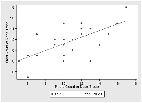
Page 76, figure 3.5
graph twoway (scatter field photo) (lfit field photo), ylabel(6(2)18, nogrid angle(0)) ///
  ytitle(Field Count of Dead Trees) xtitle(Photo Count of Dead Trees) xlabel(6(2)18)
Page 79 in the middle
use https://stats.idre.ucla.edu/stat/stata/examples/lohr/agsrs.dta, clear
gen west = 0
replace west = 1 if state =="AK" | state =="AZ" | state =="CA" | state =="CO" | state =="HI" | ///
  state =="ID" | state =="MT" | state =="NV" | state =="NM" | state =="OR" | state =="UT" | ///
  state =="WA" | state =="WY"
drop if west == 0
tabstat acres92, s(mean sd)

    variable |      mean        sd
-------------+--------------------
     acres92 |  598680.6  516157.7
----------------------------------
Page 83 at the bottom
NOTE: The three values that are predicted after the svy: reg
command are used for the table on the next page.NOTE: You need to
update Stata 9 before this will run without an error message. To
update your Stata, (while on the internet) type: update all.
use https://stats.idre.ucla.edu/stat/stata/examples/lohr/agsrs.dta, clear
gen wt = 1/acres87
svyset [pweight = wt]
svy: reg acres92 acres87, nocons
predict yhat
predict sterror, stdp
predict residual, resid

Survey linear regression
pweight:  wt                                      Number of obs    =       299
Strata:   <one>                                   Number of strata =         1
PSU:      <observations>                          Number of PSUs   =       299
                                                  Population size  = .00759475
                                                  F(   1,    298)  =  26564.60
                                                  Prob > F         =    0.0000
                                                  R-squared        =    0.9929
------------------------------------------------------------------------------
     acres92 |      Coef.   Std. Err.      t    P>|t|     [95% Conf. Interval]
-------------+----------------------------------------------------------------
     acres87 |   .9865652    .006053   162.99   0.000     .9746531    .9984774
------------------------------------------------------------------------------
Page 84 at the top
NOTE: It is unclear what two line were added to the bottom of the SAS
data file. Also, Appendix E is table of random numbers.
list wt acres92 yhat sterror residual in 1/10

     +------------------------------------------------------+
     |       wt   acres92       yhat    sterror    residual |
     |------------------------------------------------------|
  1. | 5.58e-06    175209     176902   1085.378   -1692.999 |
  2. | 6.89e-06    138135   143154.6   878.3216   -5019.562 |
  3. | .0000167     56102   59056.78   362.3416   -2954.782 |
  4. | 4.53e-06    199117   217563.3   1334.855   -18446.29 |
  5. | 9.47e-06     89228   104167.5   639.1172   -14939.48 |
     |------------------------------------------------------|
  6. | 8.30e-06     96194   118922.5   729.6466   -22728.55 |
  7. | .0000151     57253   65414.21   401.3474   -8161.208 |
  8. | 4.47e-06    210692   220590.1   1353.425   -9898.067 |
  9. | .0000125     78498   79188.63     485.86   -690.6319 |
 10. | 4.26e-06    219444   231453.1   1420.075   -12009.14 |
     +------------------------------------------------------+

list wt acres92 yhat sterror residual in -4/l

     +------------------------------------------------------+
     |       wt   acres92       yhat    sterror    residual |
     |------------------------------------------------------|
297. | 2.80e-06    343115   352944.7   2165.484     -9829.7 |
298. | .0000468     19956   21081.91   129.3476   -1125.913 |
299. | .0000636     15650   15504.86   95.12971    145.1407 |
300. |  .000018     55827   54887.56   336.7614     939.443 |
     +------------------------------------------------------+
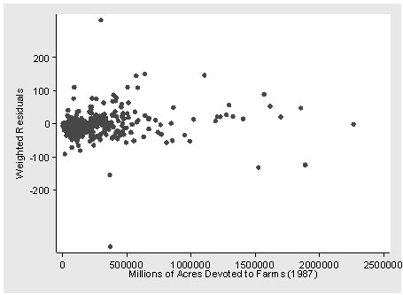
Page 85, figure 3.6
NOTE: Although the title is shown on the graph below as it is in the
text, the scale of the x-axis was not changed as it was in the text.
gen wtdresid = (acres92 - .986565*acres87)/sqrt(acres87)
graph scatter wtdresid acres87, ylabel(-200(100)200, angle(0) nogrid) ytitle(Weighted Residuals) ///
  xtitle("Millions of Acres Devoted to Farms (1987)")