
Note: This chapter uses a suite of commands, called spost, written by
J. Scott Long and Jeremy Freese. The commands must be downloaded prior to
their use, and this can be done by typing search spost in the Stata command
line (see How can I use the search command to
search for programs and get additional help? for more information about
using search).
Table 7.1, page 191.
use https://stats.idre.ucla.edu/stat/stata/examples/long/tobjob2, clear

quietly reg jobcen fem phd ment fel art cit
listcoef, std

regress (N=408): Unstandardized and Standardized Estimates

 Observed SD: .97360294
 SD of Error: .8717482

-------------------------------------------------------------------------------
      jobcen |      b         t     P>|t|    bStdX    bStdY   bStdXY      SDofX
-------------+-----------------------------------------------------------------
         fem |  -0.13919   -1.543   0.124  -0.0680  -0.1430  -0.0698     0.4883
         phd |   0.27268    5.529   0.000   0.2601   0.2801   0.2671     0.9538
        ment |   0.00119    1.692   0.091   0.0778   0.0012   0.0799    65.5299
         fel |   0.23414    2.469   0.014   0.1139   0.2405   0.1170     0.4866
         art |   0.02280    0.789   0.430   0.0514   0.0234   0.0528     2.2561
         cit |   0.00448    2.275   0.023   0.1481   0.0046   0.1521    33.0599
-------------------------------------------------------------------------------

quietly reg jobcen fem phd ment fel art cit if jobcen ~= 1
listcoef, std

regress (N=309): Unstandardized and Standardized Estimates

 Observed SD: .77904266
 SD of Error: .70309389

-------------------------------------------------------------------------------
      jobcen |      b         t     P>|t|    bStdX    bStdY   bStdXY      SDofX
-------------+-----------------------------------------------------------------
         fem |   0.10145    1.187   0.236   0.0481   0.1302   0.0618     0.4744
         phd |   0.29738    6.361   0.000   0.2758   0.3817   0.3540     0.9274
        ment |   0.00078    1.273   0.204   0.0541   0.0010   0.0695    69.5468
         fel |   0.14053    1.565   0.119   0.0662   0.1804   0.0850     0.4710
         art |   0.00590    0.238   0.812   0.0142   0.0076   0.0182     2.4000
         cit |   0.00210    1.271   0.205   0.0760   0.0027   0.0976    36.1466
-------------------------------------------------------------------------------

quietly tobit jobcen fem phd ment fel art cit, ll(1)
listcoef, std

tobit (N=408): Unstandardized and Standardized Estimates

 Observed SD: .97360294
   Latent SD: 1.21966
 SD of Error: 1.087237

-------------------------------------------------------------------------------
      jobcen |      b         t     P>|t|    bStdX    bStdY   bStdXY      SDofX
-------------+-----------------------------------------------------------------
         fem |  -0.23685   -2.032   0.043  -0.1156  -0.1942  -0.0948     0.4883
         phd |   0.32258    5.047   0.000   0.3077   0.2645   0.2523     0.9538
        ment |   0.00134    1.514   0.131   0.0880   0.0011   0.0722    65.5299
         fel |   0.32527    2.656   0.008   0.1583   0.2667   0.1298     0.4866
         art |   0.03391    0.929   0.353   0.0765   0.0278   0.0627     2.2561
         cit |   0.00509    2.057   0.040   0.1683   0.0042   0.1380    33.0599
-------------------------------------------------------------------------------
Figure 7.6, page 200.
Note: This graph was created in three steps since the prgen command after
tobit produces expected values rather than probabilities.
Step 1: Create a data set for each of the categories, female fellow (ff),
female nonfellow(fnf), male fellow(mf) and male nonfellow(mnf) where the level
of PhD varies from 1 to 5 by .5 and the other variables in the model, ment,
art and cit are held at there mean. The four data sets where
created from the data set figure76
where for each respective data set, fem
and fel where varied to define each case type.
Step 2: Run the full tobit model and use that model for out-of-sample
prediction for the four data sets, ff, fnf, mf and mnf, where we predict the
probability of being censored with the command predict varname, pr(.,1)
as well as sorting the observations.
Step 3: Merge all the data sets together by the phd variable and graph
the probability of censor to phd level.
Step 1.
clear
input phd
1
1.5
2
2.5
3
3.5
4
4.5
5
end

gen ment = 45.47058
gen art = 2.276961
gen cit = 21.71569
save figure76
file figure76.dta saved

*create data for female fellow
use figure76
gen fem =1
gen fel =1
save ff
file ff.dta saved

*create data for female nonfellow
use figure76
gen fem =1
gen fel =0
save fnf
file fnf.dta saved

*create data for male fellow
use figure76
gen fem =0
gen fel =1
save mf
file mf.dta saved

*create data for male nonfellow
use figure76
gen fem =0
gen fel =0
save mnf
file mnf.dta saved
Step 2.
use https://stats.idre.ucla.edu/stat/stata/examples/long/tobjob2, clear
(Academic Biochemists / S Long)

quietly tobit jobcen fem phd ment fel art cit, ll(1)
use ff, clear
predict ffcen, pr(.,1)
label var ffcen "female fellow"
sort phd
save ff, replace
file ff.dta saved

use fnf, clear
predict fnfcen, pr(.,1)
label var fnfcen "female nonfellow"
sort phd
save fnf,replace
file fnf.dta saved

use mf, clear
predict mfcen, pr(.,1)
label var mfcen "male fellow"
sort phd
save mf,replace
file mf.dta saved

use mnf, clear
predict mnfcen, pr(.,1)
label var mnfcen "male nonfellow"
sort phd
save mnf,replace
file mnf.dta saved

use ff, clear
merge phd using fnf mf mnf
graph twoway (scatter ffcen fnfcen mfcen mnfcen phd, c(l l l l) ///
	xtitle("Ph.D. Prestige") ytitle("Pr(Censored)"))
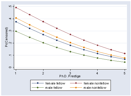
Table 7.1, page 215. Hausman and Wise’s OLS and ML Estimates From a Sample With Truncation.
NOTE: This has been skipped because we do not have the data.