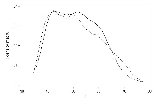
use https://stats.idre.ucla.edu/stat/stata/examples/methods_matter/chapter12/catholic, clear
Descriptive statistics for mathematics score (math12) and
type of high school (catholic). Note: this output does not
appear in the text.
sum math12 catholic, detail

          12th grade standardized mathematics score
-------------------------------------------------------------
      Percentiles      Smallest
 1%        32.88          29.88
 5%        35.46          30.14
10%        37.54          30.42       Obs                5671
25%        43.53          30.55       Sum of Wgt.        5671

50%        51.33                      Mean           51.05124
                        Largest       Std. Dev.      9.502415
75%        58.61          70.94
90%        63.67          71.08       Variance        90.2959
95%        65.98          71.12       Skewness      -.0567201
99%        69.33          71.37       Kurtosis       2.072073

                    attended catholic hs?
-------------------------------------------------------------
      Percentiles      Smallest
 1%            0              0
 5%            0              0
10%            0              0       Obs                5671
25%            0              0       Sum of Wgt.        5671

50%            0                      Mean           .1043908
                        Largest       Std. Dev.      .3057938
75%            0              1
90%            1              1       Variance       .0935098
95%            1              1       Skewness       2.587653
99%            1              1       Kurtosis        7.69595

table catholic, contents(mean math12 sd math12 freq)

----------------------------------------------------
attended  |
catholic  |
hs?       | mean(math12)    sd(math12)         Freq.
----------+-----------------------------------------
       no |     50.64465      9.534295         5,079
      yes |     54.53951      8.463153           592
----------------------------------------------------
Descriptive statistics for family income (faminc8). (Not shown in text.)
sum faminc8, detail

           total annual family income in 8th grade
-------------------------------------------------------------
      Percentiles      Smallest
 1%            2              1
 5%            5              1
10%            7              1       Obs                5671
25%            8              1       Sum of Wgt.        5671

50%           10                      Mean           9.526186
                        Largest       Std. Dev.      2.217688
75%           11             12
90%           12             12       Variance       4.918141
95%           12             12       Skewness      -1.268464
99%           12             12       Kurtosis       4.447905
Various methods of examining the relationship between catholic
and faminc8. (Not shown in text.)
by catholic, sort: sum faminc8, detail

------------------------------------------------------------------------------------------------------
-> catholic = no

           total annual family income in 8th grade
-------------------------------------------------------------
      Percentiles      Smallest
 1%            2              1
 5%            5              1
10%            6              1       Obs                5079
25%            8              1       Sum of Wgt.        5079

50%           10                      Mean           9.428825
                        Largest       Std. Dev.       2.25239
75%           11             12
90%           12             12       Variance       5.073261
95%           12             12       Skewness      -1.214205
99%           12             12       Kurtosis       4.255522

------------------------------------------------------------------------------------------------------
-> catholic = yes

           total annual family income in 8th grade
-------------------------------------------------------------
      Percentiles      Smallest
 1%            4              1
 5%            7              2
10%            8              4       Obs                 592
25%           10              4       Sum of Wgt.         592

50%           11                      Mean           10.36149
                        Largest       Std. Dev.       1.67728
75%           11             12
90%           12             12       Variance       2.813269
95%           12             12       Skewness      -1.784059
99%           12             12       Kurtosis       7.343344


tab faminc8 catholic, chi2

   total annual |
  family income | attended catholic hs?
   in 8th grade |        no        yes |     Total
----------------+----------------------+----------
           none |        17          1 |        18
         <$1000 |        41          1 |        42
    $1000-$2999 |        84          0 |        84
    $3000-$4999 |        79          6 |        85
    $5000-$7499 |       138          6 |       144
     7500-$9999 |       169          6 |       175
  $10000-$14999 |       427         20 |       447
  $15000-$19999 |       410         31 |       441
  $20000-$24999 |       608         47 |       655
  $25000-$34999 |     1,137        130 |     1,267
   35000-$49999 |     1,221        198 |     1,419
   50000-$74999 |       748        146 |       894
----------------+----------------------+----------
          Total |     5,079        592 |     5,671

         Pearson chi2(11) = 111.4057   Pr = 0.000

pwcorr faminc8 catholic, sig

             |  faminc8 catholic
-------------+------------------
     faminc8 |   1.0000
             |
             |
    catholic |   0.1286   1.0000
             |   0.0000
             |
Categorize faminc8 into catfaminc8, and examine the relationship between the two variables.
(Not shown in text.)
egen catfaminc8=cut(faminc8), at(1,9,11,13) icodes

tab catfaminc8

 catfaminc8 |      Freq.     Percent        Cum.
------------+-----------------------------------
          0 |      1,436       25.32       25.32
          1 |      1,922       33.89       59.21
          2 |      2,313       40.79      100.00
------------+-----------------------------------
      Total |      5,671      100.00

tab faminc8 catfaminc8

   total annual |
  family income |            catfaminc8
   in 8th grade |         0          1          2 |     Total
----------------+---------------------------------+----------
           none |        18          0          0 |        18
         <$1000 |        42          0          0 |        42
    $1000-$2999 |        84          0          0 |        84
    $3000-$4999 |        85          0          0 |        85
    $5000-$7499 |       144          0          0 |       144
     7500-$9999 |       175          0          0 |       175
  $10000-$14999 |       447          0          0 |       447
  $15000-$19999 |       441          0          0 |       441
  $20000-$24999 |         0        655          0 |       655
  $25000-$34999 |         0      1,267          0 |     1,267
   35000-$49999 |         0          0      1,419 |     1,419
   50000-$74999 |         0          0        894 |       894
----------------+---------------------------------+----------
          Total |     1,436      1,922      2,313 |     5,671
Table 12.1 on page 293.
* Sample variance of faminc8 in each income category.
tabstat faminc8, by(catfaminc8) statistics(var)

Summary for variables: faminc8
     by categories of: catfaminc8

catfaminc8 |  variance
-----------+----------
         0 |  3.063001
         1 |  .2247694
         2 |  .2372228
-----------+----------
     Total |  4.918141
----------------------

* Sample mean of faminc8 by income category and school type.
table catfaminc8 catholic, contents(mean faminc8)

------------------------------------------
catfaminc |     attended catholic hs?
8         |             no             yes
----------+-------------------------------
        0 |  6.32967042923  6.774647712708
        1 | 9.651576042175  9.734463691711
        2 | 11.37988853455   11.4244184494
------------------------------------------

* Tests for differences in family income by school type within each income category.
by catfaminc8, sort : ttest faminc8, by(catholic)

------------------------------------------------------------------------------------------------------
-> catfaminc8 = 0

Two-sample t test with equal variances
------------------------------------------------------------------------------
Variable |     Obs        Mean    Std. Err.   Std. Dev.   [95% Conf. Interval]
---------+--------------------------------------------------------------------
      no |    1365     6.32967    .0475499    1.756773    6.236392    6.422949
     yes |      71    6.774648    .1862445    1.569324    6.403195    7.146101
---------+--------------------------------------------------------------------
combined |    1436    6.351671    .0461845    1.750143    6.261075    6.442268
---------+--------------------------------------------------------------------
    diff |           -.4449776    .2127872               -.8623851   -.0275701
------------------------------------------------------------------------------
    diff = mean(no) - mean(yes)                                   t =  -2.0912
Ho: diff = 0                                     degrees of freedom =     1434

    Ha: diff < 0                 Ha: diff != 0                 Ha: diff > 0
 Pr(T < t) = 0.0183         Pr(|T| > |t|) = 0.0367          Pr(T > t) = 0.9817

------------------------------------------------------------------------------------------------------
-> catfaminc8 = 1

Two-sample t test with equal variances
------------------------------------------------------------------------------
Variable |     Obs        Mean    Std. Err.   Std. Dev.   [95% Conf. Interval]
---------+--------------------------------------------------------------------
      no |    1745    9.651576    .0114094    .4766077    9.629198    9.673954
     yes |     177    9.734463    .0332883    .4428714    9.668768    9.800159
---------+--------------------------------------------------------------------
combined |    1922    9.659209    .0108141    .4740985       9.638    9.680418
---------+--------------------------------------------------------------------
    diff |           -.0828873     .037361               -.1561597    -.009615
------------------------------------------------------------------------------
    diff = mean(no) - mean(yes)                                   t =  -2.2186
Ho: diff = 0                                     degrees of freedom =     1920

    Ha: diff < 0                 Ha: diff != 0                 Ha: diff > 0
 Pr(T < t) = 0.0133         Pr(|T| > |t|) = 0.0266          Pr(T > t) = 0.9867

------------------------------------------------------------------------------------------------------
-> catfaminc8 = 2

Two-sample t test with equal variances
------------------------------------------------------------------------------
Variable |     Obs        Mean    Std. Err.   Std. Dev.   [95% Conf. Interval]
---------+--------------------------------------------------------------------
      no |    1969    11.37989    .0109408    .4854821    11.35843    11.40135
     yes |     344    11.42442    .0266872    .4949744    11.37193    11.47691
---------+--------------------------------------------------------------------
combined |    2313    11.38651    .0101272    .4870552    11.36665    11.40637
---------+--------------------------------------------------------------------
    diff |           -.0445303     .028453               -.1003264    .0112657
------------------------------------------------------------------------------
    diff = mean(no) - mean(yes)                                   t =  -1.5650
Ho: diff = 0                                     degrees of freedom =     2311

    Ha: diff < 0                 Ha: diff != 0                 Ha: diff > 0
 Pr(T < t) = 0.0589         Pr(|T| > |t|) = 0.1177          Pr(T > t) = 0.9411


tab catfaminc8 catholic, row

+----------------+
| Key            |
|----------------|
|   frequency    |
| row percentage |
+----------------+

           | attended catholic hs?
catfaminc8 |        no        yes |     Total
-----------+----------------------+----------
         0 |     1,365         71 |     1,436
           |     95.06       4.94 |    100.00
-----------+----------------------+----------
         1 |     1,745        177 |     1,922
           |     90.79       9.21 |    100.00
-----------+----------------------+----------
         2 |     1,969        344 |     2,313
           |     85.13      14.87 |    100.00
-----------+----------------------+----------
     Total |     5,079        592 |     5,671
           |     89.56      10.44 |    100.00


* Average math achievement, by school type and income category.
table catfaminc8 catholic, contents(mean math12)

------------------------------
          | attended catholic
catfaminc |        hs?
8         |       no       yes
----------+-------------------
        0 | 46.77358  50.53563
        1 | 50.33842  53.85616
        2 | 53.59964   55.7175
------------------------------

* Tests for differences in average math achievement by school type within each income category.
by catfaminc8, sort : ttest math12, by(catholic)

------------------------------------------------------------------------------------------------------
-> catfaminc8 = 0

Two-sample t test with equal variances
------------------------------------------------------------------------------
Variable |     Obs        Mean    Std. Err.   Std. Dev.   [95% Conf. Interval]
---------+--------------------------------------------------------------------
      no |    1365    46.77358    .2409728     8.90296    46.30086     47.2463
     yes |      71    50.53563    1.003933    8.459293    48.53335    52.53792
---------+--------------------------------------------------------------------
combined |    1436    46.95959    .2352876    8.916128    46.49804    47.42113
---------+--------------------------------------------------------------------
    diff |           -3.762051    1.081144               -5.882845   -1.641258
------------------------------------------------------------------------------
    diff = mean(no) - mean(yes)                                   t =  -3.4797
Ho: diff = 0                                     degrees of freedom =     1434

    Ha: diff < 0                 Ha: diff != 0                 Ha: diff > 0
 Pr(T < t) = 0.0003         Pr(|T| > |t|) = 0.0005          Pr(T > t) = 0.9997

------------------------------------------------------------------------------------------------------
-> catfaminc8 = 1

Two-sample t test with equal variances
------------------------------------------------------------------------------
Variable |     Obs        Mean    Std. Err.   Std. Dev.   [95% Conf. Interval]
---------+--------------------------------------------------------------------
      no |    1745    50.33842    .2228944    9.311012    49.90126    50.77559
     yes |     177    53.85616    .6445502    8.575183    52.58412     55.1282
---------+--------------------------------------------------------------------
combined |    1922    50.66238    .2121188    9.299418    50.24637    51.07838
---------+--------------------------------------------------------------------
    diff |           -3.517734    .7293671               -4.948169   -2.087299
------------------------------------------------------------------------------
    diff = mean(no) - mean(yes)                                   t =  -4.8230
Ho: diff = 0                                     degrees of freedom =     1920

    Ha: diff < 0                 Ha: diff != 0                 Ha: diff > 0
 Pr(T < t) = 0.0000         Pr(|T| > |t|) = 0.0000          Pr(T > t) = 1.0000

------------------------------------------------------------------------------------------------------
-> catfaminc8 = 2

Two-sample t test with equal variances
------------------------------------------------------------------------------
Variable |     Obs        Mean    Std. Err.   Std. Dev.   [95% Conf. Interval]
---------+--------------------------------------------------------------------
      no |    1969    53.59964    .2060271    9.142124    53.19559    54.00369
     yes |     344     55.7175    .4384348    8.131754    54.85514    56.57986
---------+--------------------------------------------------------------------
combined |    2313    53.91462    .1877359    9.028905    53.54647    54.28277
---------+--------------------------------------------------------------------
    diff |           -2.117861    .5258916               -3.149129   -1.086592
------------------------------------------------------------------------------
    diff = mean(no) - mean(yes)                                   t =  -4.0272
Ho: diff = 0                                     degrees of freedom =     2311

    Ha: diff < 0                 Ha: diff != 0                 Ha: diff > 0
 Pr(T < t) = 0.0000         Pr(|T| > |t|) = 0.0001          Pr(T > t) = 1.0000
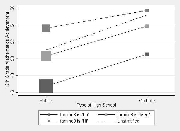
Figure 12.1 on page 297.
sort catholic catfaminc8
by catholic catfaminc8: egen n = count(id)
by catholic catfaminc8: egen mmath12 = mean(math12)

twoway (scatter mmath12 catholic [aweight=n] if catfaminc8==0, connect(l) msymbol(S)) ///
	(scatter mmath12 catholic [aweight=n] if catfaminc8==1, connect(l) msymbol(S)) ///
	(scatter mmath12 catholic [aweight=n] if catfaminc8==2, connect(l) msymbol(S)) ///
	(lfit math12 catholic [aweight=n]),     ///
	xlabel(0 "Public" 1 "Catholic") xscale(range(-.25 1.25)) ///
	legend(label(1 `"faminc8 is "Lo""') label(2 `"faminc8 is "Med""') ///
	label(3 `"faminc8 is "Hi""') label(4 `"Unstratified"')) ///
	xtitle("Type of High School") ytitle("12rh Grade Mathematics Achievement") ///
	scheme(s2mono)
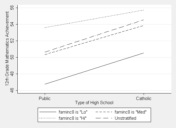
A simplified graph that provides information similar to that in
Figure 12.1 can be produced using the syntax shown below. (Not shown in the text.)
twoway  (lfit math12 catholic if catfaminc8==0) ///
	(lfit math12 catholic if catfaminc8==1) ///
	(lfit math12 catholic if catfaminc8==2) ///
	(lfit math12 catholic), ///
	xlabel(0 "Public" 1 "Catholic") xscale(range(-.25 1.25)) ///
	legend(label(1 `"faminc8 is "Lo""') label(2 `"faminc8 is "Med""') ///
	label(3 `"faminc8 is "Hi""') label(4 `"Unstratified"')) ///
	xtitle("Type of High School") ytitle("12rh Grade Mathematics Achievement") ///
	scheme(s2mono)
OLS regression model of math12 on catholic. This
regression corresponds to the "Unstratified" line in Figure 12.1. (Not shown in the text.)
regress  math12 catholic

      Source |       SS       df       MS              Number of obs =    5671
-------------+------------------------------           F(  1,  5669) =   90.48
       Model |   8043.1077     1   8043.1077           Prob > F      =  0.0000
    Residual |  503934.635  5669  88.8930385           R-squared     =  0.0157
-------------+------------------------------           Adj R-squared =  0.0155
       Total |  511977.743  5670  90.2958982           Root MSE      =  9.4283

------------------------------------------------------------------------------
      math12 |      Coef.   Std. Err.      t    P>|t|     [95% Conf. Interval]
-------------+----------------------------------------------------------------
    catholic |    3.89486   .4094621     9.51   0.000     3.092157    4.697562
       _cons |   50.64465   .1322954   382.81   0.000      50.3853      50.904
------------------------------------------------------------------------------
OLS regression of math12 on catholic, stratifying by
catfaminc8. These
regressions correspond to the information shown in Figure 12.1. (Not shown in text.)
by catfaminc8, sort: regress  math12 catholic

------------------------------------------------------------------------------------------------------
-> catfaminc8 = 0

      Source |       SS       df       MS              Number of obs =    1436
-------------+------------------------------           F(  1,  1434) =   12.11
       Model |  955.181769     1  955.181769           Prob > F      =  0.0005
    Residual |  113123.499  1434  78.8866802           R-squared     =  0.0084
-------------+------------------------------           Adj R-squared =  0.0077
       Total |  114078.681  1435  79.4973388           Root MSE      =  8.8818

------------------------------------------------------------------------------
      math12 |      Coef.   Std. Err.      t    P>|t|     [95% Conf. Interval]
-------------+----------------------------------------------------------------
    catholic |   3.762051   1.081144     3.48   0.001     1.641258    5.882845
       _cons |   46.77358   .2404006   194.57   0.000     46.30201    47.24516
------------------------------------------------------------------------------

------------------------------------------------------------------------------------------------------
-> catfaminc8 = 1

      Source |       SS       df       MS              Number of obs =    1922
-------------+------------------------------           F(  1,  1920) =   23.26
       Model |  1988.57183     1  1988.57183           Prob > F      =  0.0000
    Residual |  164137.924  1920  85.4885019           R-squared     =  0.0120
-------------+------------------------------           Adj R-squared =  0.0115
       Total |  166126.496  1921  86.4791752           Root MSE      =   9.246

------------------------------------------------------------------------------
      math12 |      Coef.   Std. Err.      t    P>|t|     [95% Conf. Interval]
-------------+----------------------------------------------------------------
    catholic |   3.517734   .7293671     4.82   0.000     2.087299    4.948169
       _cons |   50.33842   .2213381   227.43   0.000     49.90434    50.77251
------------------------------------------------------------------------------

------------------------------------------------------------------------------------------------------
-> catfaminc8 = 2

      Source |       SS       df       MS              Number of obs =    2313
-------------+------------------------------           F(  1,  2311) =   16.22
       Model |  1313.47946     1  1313.47946           Prob > F      =  0.0001
    Residual |  187163.381  2311  80.9880488           R-squared     =  0.0070
-------------+------------------------------           Adj R-squared =  0.0065
       Total |   188476.86  2312  81.5211333           Root MSE      =  8.9993

------------------------------------------------------------------------------
      math12 |      Coef.   Std. Err.      t    P>|t|     [95% Conf. Interval]
-------------+----------------------------------------------------------------
    catholic |   2.117861   .5258916     4.03   0.000     1.086592    3.149129
       _cons |   53.59964   .2028092   264.29   0.000     53.20193    53.99735
------------------------------------------------------------------------------
Descriptive statistics for math achievement (math8).
(Not shown in text.)
sum math8, detail

          8th grade standardized mathematics score
-------------------------------------------------------------
      Percentiles      Smallest
 1%        35.95          34.48
 5%        37.89          34.49
10%        39.42          34.52       Obs                5671
25%        43.45          34.52       Sum of Wgt.        5671

50%        50.45                      Mean           51.48952
                        Largest       Std. Dev.      9.683425
75%        58.56           77.2
90%        65.39           77.2       Variance       93.76872
95%        68.89           77.2       Skewness       .4078902
99%        74.04           77.2       Kurtosis       2.319295
Several methods of examining the relationship between
math8 and catholic. (Not shown in text.)
corr math8 catholic
(obs=5671)

             |    math8 catholic
-------------+------------------
       math8 |   1.0000
    catholic |   0.0765   1.0000


ttest math8, by(catholic)

Two-sample t test with equal variances
------------------------------------------------------------------------------
Variable |     Obs        Mean    Std. Err.   Std. Dev.   [95% Conf. Interval]
---------+--------------------------------------------------------------------
      no |    5079    51.23648    .1367773    9.747724    50.96834    51.50462
     yes |     592    53.66039    .3628002     8.82731    52.94785    54.37292
---------+--------------------------------------------------------------------
combined |    5671    51.48952    .1285876    9.683425    51.23743     51.7416
---------+--------------------------------------------------------------------
    diff |           -2.423907    .4193447               -3.245983   -1.601831
------------------------------------------------------------------------------
    diff = mean(no) - mean(yes)                                   t =  -5.7802
Ho: diff = 0                                     degrees of freedom =     5669

    Ha: diff < 0                 Ha: diff != 0                 Ha: diff > 0
 Pr(T < t) = 0.0000         Pr(|T| > |t|) = 0.0000          Pr(T > t) = 1.0000
Create a categorical variable for prior math achievement (catmath8), and
examine the relationship between cathmath8 and math8. (Not shown
in text.)
egen catmath8=cut(math8), at(30,38,44,51,80) icodes
tab catmath8

   catmath8 |      Freq.     Percent        Cum.
------------+-----------------------------------
          0 |        304        5.36        5.36
          1 |      1,236       21.80       27.16
          2 |      1,421       25.06       52.21
          3 |      2,710       47.79      100.00
------------+-----------------------------------
      Total |      5,671      100.00


table catmath8, contents(mean math8 sd math8 freq)

-------------------------------------------------
 catmath8 | mean(math8)    sd(math8)        Freq.
----------+--------------------------------------
        0 |    36.78859     .8564365          304
        1 |    41.10199     1.722423        1,236
        2 |    47.53923     2.045117        1,421
        3 |     59.9476      6.27689        2,710
-------------------------------------------------
Check for balance in math8 within strata
(catmath8), by catholic. (Not shown in the text.)
table catmath8 catholic, contents(mean math8 sd math8 freq)

------------------------------
          | attended catholic
          |        hs?
 catmath8 |       no       yes
----------+-------------------
        0 | 36.80332  36.30556
          | .8559109  .7666504
          |      295         9
          |
        1 | 41.09058   41.2438
          | 1.718102  1.778788
          |    1,144        92
          |
        2 | 47.49826  47.92955
          | 2.040288  2.057497
          |    1,286       135
          |
        3 | 60.01815  59.48112
          | 6.348762  5.765806
          |    2,354       356
------------------------------

by catmath8, sort : ttest math8, by(catholic)

------------------------------------------------------------------------------------------------------
-> catmath8 = 0

Two-sample t test with equal variances
------------------------------------------------------------------------------
Variable |     Obs        Mean    Std. Err.   Std. Dev.   [95% Conf. Interval]
---------+--------------------------------------------------------------------
      no |     295    36.80332    .0498331    .8559109    36.70525     36.9014
     yes |       9    36.30556    .2555501    .7666504    35.71626    36.89486
---------+--------------------------------------------------------------------
combined |     304    36.78859      .04912    .8564365    36.69193    36.88525
---------+--------------------------------------------------------------------
    diff |            .4977666    .2888636               -.0706738    1.066207
------------------------------------------------------------------------------
    diff = mean(no) - mean(yes)                                   t =   1.7232
Ho: diff = 0                                     degrees of freedom =      302

    Ha: diff < 0                 Ha: diff != 0                 Ha: diff > 0
 Pr(T < t) = 0.9571         Pr(|T| > |t|) = 0.0859          Pr(T > t) = 0.0429

------------------------------------------------------------------------------------------------------
-> catmath8 = 1

Two-sample t test with equal variances
------------------------------------------------------------------------------
Variable |     Obs        Mean    Std. Err.   Std. Dev.   [95% Conf. Interval]
---------+--------------------------------------------------------------------
      no |    1144    41.09059    .0507967    1.718102    40.99092    41.19025
     yes |      92     41.2438    .1854515    1.778788    40.87543    41.61218
---------+--------------------------------------------------------------------
combined |    1236    41.10199    .0489926    1.722423    41.00587    41.19811
---------+--------------------------------------------------------------------
    diff |           -.1532187    .1866807               -.5194654     .213028
------------------------------------------------------------------------------
    diff = mean(no) - mean(yes)                                   t =  -0.8208
Ho: diff = 0                                     degrees of freedom =     1234

    Ha: diff < 0                 Ha: diff != 0                 Ha: diff > 0
 Pr(T < t) = 0.2060         Pr(|T| > |t|) = 0.4119          Pr(T > t) = 0.7940

------------------------------------------------------------------------------------------------------
-> catmath8 = 2

Two-sample t test with equal variances
------------------------------------------------------------------------------
Variable |     Obs        Mean    Std. Err.   Std. Dev.   [95% Conf. Interval]
---------+--------------------------------------------------------------------
      no |    1286    47.49826    .0568946    2.040288    47.38664    47.60987
     yes |     135    47.92956    .1770811    2.057497    47.57932    48.27979
---------+--------------------------------------------------------------------
combined |    1421    47.53923    .0542527    2.045117    47.43281    47.64566
---------+--------------------------------------------------------------------
    diff |           -.4312974    .1847346               -.7936796   -.0689152
------------------------------------------------------------------------------
    diff = mean(no) - mean(yes)                                   t =  -2.3347
Ho: diff = 0                                     degrees of freedom =     1419

    Ha: diff < 0                 Ha: diff != 0                 Ha: diff > 0
 Pr(T < t) = 0.0098         Pr(|T| > |t|) = 0.0197          Pr(T > t) = 0.9902

------------------------------------------------------------------------------------------------------
-> catmath8 = 3

Two-sample t test with equal variances
------------------------------------------------------------------------------
Variable |     Obs        Mean    Std. Err.   Std. Dev.   [95% Conf. Interval]
---------+--------------------------------------------------------------------
      no |    2354    60.01815    .1308536    6.348762    59.76155    60.27475
     yes |     356    59.48112    .3055871    5.765806    58.88013    60.08211
---------+--------------------------------------------------------------------
combined |    2710     59.9476    .1205757     6.27689    59.71117    60.18403
---------+--------------------------------------------------------------------
    diff |            .5370243    .3568614               -.1627239    1.236773
------------------------------------------------------------------------------
    diff = mean(no) - mean(yes)                                   t =   1.5049
Ho: diff = 0                                     degrees of freedom =     2708

    Ha: diff < 0                 Ha: diff != 0                 Ha: diff > 0
 Pr(T < t) = 0.9338         Pr(|T| > |t|) = 0.1325          Pr(T > t) = 0.0662
Table 12.1 on page 301.
table catmath8 catholic , contents(mean math12 freq) by(catfaminc8)

------------------------------
catfaminc | attended catholic
8 and     |        hs?
catmath8  |       no       yes
----------+-------------------
0         |
        0 | 36.80514     42.57
          |      142         1
          |
        1 | 40.99247   41.7019
          |      433        21
          |
        2 | 47.12156  48.65308
          |      385        13
          |
        3 | 56.11869  56.58972
          |      405        36
----------+-------------------
1         |
        0 | 37.94156    39.775
          |       96         2
          |
        1 | 41.92456  44.56454
          |      390        33
          |
        2 |  47.9487  50.13551
          |      469        49
          |
        3 | 57.41727  59.41634
          |      790        93
----------+-------------------
2         |
        0 | 39.78667  40.40334
          |       57         6
          |
        1 |  42.7458  44.22737
          |      321        38
          |
        2 | 49.17894  50.70644
          |      432        73
          |
        3 | 58.93283  59.65723
          |    1,159       227
------------------------------
The t-tests shown in Table 12.1 on page 301 can be reproduced
using the following syntax. (Note: most of the output was omitted to
save space.)
bysort catfaminc8 catmath8: ttest math12, by(catholic)

------------------------------------------------------------------------------------------------------
-> catfaminc8 = 0, catmath8 = 0

Two-sample t test with equal variances
------------------------------------------------------------------------------
Variable |     Obs        Mean    Std. Err.   Std. Dev.   [95% Conf. Interval]
---------+--------------------------------------------------------------------
      no |     142    36.80514    .3391017    4.040863    36.13476    37.47552
     yes |       1       42.57           .           .           .           .
---------+--------------------------------------------------------------------
combined |     143    36.84545           .           .           .           .
---------+--------------------------------------------------------------------
    diff |           -5.764859           .                       .           .
------------------------------------------------------------------------------
    diff = mean(no) - mean(yes)                                   t =        .
Ho: diff = 0                                     degrees of freedom =      141

    Ha: diff < 0                 Ha: diff != 0                 Ha: diff > 0
 Pr(T < t) =      .         Pr(|T| > |t|) =      .          Pr(T > t) =      .

------------------------------------------------------------------------------------------------------
-> catfaminc8 = 0, catmath8 = 1

Two-sample t test with equal variances
------------------------------------------------------------------------------
Variable |     Obs        Mean    Std. Err.   Std. Dev.   [95% Conf. Interval]
---------+--------------------------------------------------------------------
      no |     433    40.99247    .2466134    5.131692    40.50776    41.47718
     yes |      21     41.7019    1.018852    4.668968    39.57662    43.82719
---------+--------------------------------------------------------------------
combined |     454    41.02529    .2397602    5.108636    40.55411    41.49647
---------+--------------------------------------------------------------------
    diff |           -.7094334    1.142284               -2.954279    1.535412
------------------------------------------------------------------------------
    diff = mean(no) - mean(yes)                                   t =  -0.6211
Ho: diff = 0                                     degrees of freedom =      452

    Ha: diff < 0                 Ha: diff != 0                 Ha: diff > 0
 Pr(T < t) = 0.2674         Pr(|T| > |t|) = 0.5349          Pr(T > t) = 0.7326

------------------------------------------------------------------------------------------------------
-> catfaminc8 = 0, catmath8 = 2

Two-sample t test with equal variances
------------------------------------------------------------------------------
Variable |     Obs        Mean    Std. Err.   Std. Dev.   [95% Conf. Interval]
---------+--------------------------------------------------------------------
      no |     385    47.12156    .2927101    5.743387    46.54604    47.69707
     yes |      13    48.65308    1.413799    5.097526    45.57267    51.73348
---------+--------------------------------------------------------------------
combined |     398    47.17158    .2869264    5.724165     46.6075    47.73567
---------+--------------------------------------------------------------------
    diff |           -1.531519    1.614382                -4.70535    1.642312
------------------------------------------------------------------------------
    diff = mean(no) - mean(yes)                                   t =  -0.9487
Ho: diff = 0                                     degrees of freedom =      396

    Ha: diff < 0                 Ha: diff != 0                 Ha: diff > 0
 Pr(T < t) = 0.1717         Pr(|T| > |t|) = 0.3434          Pr(T > t) = 0.8283
Estimate the relationship between math12 and catholic separately
in each of the strata (catfaminc8 and catmath8) and save the results to a new
dataset (cathslopes2.dta). (Note: this output does not appear in the text
and most of the output was omitted to save space.)
sort catfaminc8 catmath8
statsby diff=_b[catholic] n=e(N), by(catfaminc8 catmath8) noisily sav(cathslopes2, replace): ///
	regress math12 catholic

statsby: First call to regress with data as is:

. regress math12 catholic

      Source |       SS       df       MS              Number of obs =    5671
-------------+------------------------------           F(  1,  5669) =   90.48
       Model |   8043.1077     1   8043.1077           Prob > F      =  0.0000
    Residual |  503934.635  5669  88.8930385           R-squared     =  0.0157
-------------+------------------------------           Adj R-squared =  0.0155
       Total |  511977.743  5670  90.2958982           Root MSE      =  9.4283

------------------------------------------------------------------------------
      math12 |      Coef.   Std. Err.      t    P>|t|     [95% Conf. Interval]
-------------+----------------------------------------------------------------
    catholic |    3.89486   .4094621     9.51   0.000     3.092157    4.697562
       _cons |   50.64465   .1322954   382.81   0.000      50.3853      50.904
------------------------------------------------------------------------------

statsby legend:

      command:  regress math12 catholic
         diff:  _b[catholic]
            n:  e(N)
           by:  catfaminc8 catmath8

Statsby groups

running (regress math12 catholic) on group 1

. regress math12 catholic

      Source |       SS       df       MS              Number of obs =     143
-------------+------------------------------           F(  1,   141) =    2.02
       Model |  33.0011957     1  33.0011957           Prob > F      =  0.1573
    Residual |  2302.32862   141  16.3285718           R-squared     =  0.0141
-------------+------------------------------           Adj R-squared =  0.0071
       Total |  2335.32981   142  16.4459846           Root MSE      =  4.0409

------------------------------------------------------------------------------
      math12 |      Coef.   Std. Err.      t    P>|t|     [95% Conf. Interval]
-------------+----------------------------------------------------------------
    catholic |   5.764859   4.055066     1.42   0.157    -2.251729    13.78145
       _cons |   36.80514   .3391017   108.54   0.000     36.13476    37.47552
------------------------------------------------------------------------------

running (regress math12 catholic) on group 2

. regress math12 catholic

      Source |       SS       df       MS              Number of obs =     454
-------------+------------------------------           F(  1,   452) =    0.39
       Model |  10.0803278     1  10.0803278           Prob > F      =  0.5349
    Residual |  11812.3885   452  26.1336029           R-squared     =  0.0009
-------------+------------------------------           Adj R-squared = -0.0014
       Total |  11822.4689   453  26.0981652           Root MSE      =  5.1121

------------------------------------------------------------------------------
      math12 |      Coef.   Std. Err.      t    P>|t|     [95% Conf. Interval]
-------------+----------------------------------------------------------------
    catholic |   .7094334   1.142284     0.62   0.535    -1.535412    2.954279
       _cons |   40.99247    .245672   166.86   0.000     40.50967    41.47527
------------------------------------------------------------------------------
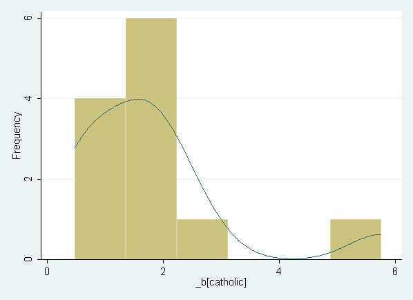
Graph the resulting slopes. Note that the entire block of
syntax should be run and once. (Not shown in the text.)
preserve
	use https://stats.idre.ucla.edu/stat/stata/examples/methods_matter/chapter12/cathslopes2, clear
	list
	histogram diff, bin(6) frequency kdensity kdenopts(gaussian)
restore

     +---------------------------------------+
     | catfam~8   catmath8       diff      n |
     |---------------------------------------|
  1. |        0          0   5.764859    143 |
  2. |        0          1   .7094334    454 |
  3. |        0          2   1.531519    398 |
  4. |        0          3    .471031    441 |
  5. |        1          0   1.833437     98 |
     |---------------------------------------|
  6. |        1          1   2.639981    423 |
  7. |        1          2   2.186811    518 |
  8. |        1          3   1.999078    883 |
  9. |        2          0   .6166673     63 |
 10. |        2          1   1.481574    359 |
     |---------------------------------------|
 11. |        2          2   1.527503    505 |
 12. |        2          3   .7243947   1386 |
     +---------------------------------------+
Similar to model A from Table 12.3 on page 306, but with dummy variables representing
the catfaminc8 by catmath8 interaction (with one group omitted as the reference category).
(Not shown in text.)
xi:  regress math12 catholic i.catfaminc8*i.catmath8
i.catfaminc8      _Icatfaminc_0-2     (naturally coded; _Icatfaminc_0 omitted)
i.catmath8        _Icatmath8_0-3      (naturally coded; _Icatmath8_0 omitted)
i.ca~c8*i.ca~h8   _IcatXcat_#_#       (coded as above)

      Source |       SS       df       MS              Number of obs =    5671
-------------+------------------------------           F( 12,  5658) =  710.06
       Model |  307674.539    12  25639.5449           Prob > F      =  0.0000
    Residual |  204303.204  5658  36.1087317           R-squared     =  0.6010
-------------+------------------------------           Adj R-squared =  0.6001
       Total |  511977.743  5670  90.2958982           Root MSE      =  6.0091

------------------------------------------------------------------------------
      math12 |      Coef.   Std. Err.      t    P>|t|     [95% Conf. Interval]
-------------+----------------------------------------------------------------
    catholic |   1.328632   .2639492     5.03   0.000     .8111899    1.846073
_Icatfamin~1 |   1.115701   .7880213     1.42   0.157    -.4291226    2.660525
_Icatfamin~2 |   2.882697   .9089585     3.17   0.002      1.10079    4.664604
_Icatmath8_1 |   4.127667   .5763251     7.16   0.000     2.997848    5.257485
_Icatmath8_2 |   10.29202    .585901    17.57   0.000     9.143432    11.44061
_Icatmath8_3 |   19.21252   .5785983    33.21   0.000     18.07825    20.34679
_IcatXca~1_1 |  -.0526632   .8865024    -0.06   0.953    -1.790548    1.685221
_IcatXca~1_2 |  -.2140083   .8840602    -0.24   0.809    -1.947105    1.519089
_IcatXca~1_3 |   .3234948   .8624064     0.38   0.708    -1.367152    2.014142
_IcatXca~2_1 |  -1.084544   1.002914    -1.08   0.280    -3.050639    .8815522
_IcatXca~2_2 |  -.8031993   .9939466    -0.81   0.419    -2.751716    1.145317
_IcatXca~2_3 |  -.0975123   .9662284    -0.10   0.920     -1.99169    1.796666
       _cons |   36.83616   .5025057    73.30   0.000     35.85106    37.82127
------------------------------------------------------------------------------
The above model can also be specified using the factor variable
syntax introduced in Stata 11.
regress math12 catholic catfaminc8##catmath8

      Source |       SS       df       MS              Number of obs =    5671
-------------+------------------------------           F( 12,  5658) =  710.06
       Model |  307674.539    12  25639.5449           Prob > F      =  0.0000
    Residual |  204303.204  5658  36.1087317           R-squared     =  0.6010
-------------+------------------------------           Adj R-squared =  0.6001
       Total |  511977.743  5670  90.2958982           Root MSE      =  6.0091

------------------------------------------------------------------------------
      math12 |      Coef.   Std. Err.      t    P>|t|     [95% Conf. Interval]
-------------+----------------------------------------------------------------
    catholic |   1.328632   .2639492     5.03   0.000     .8111899    1.846073
             |
  catfaminc8 |
          1  |   1.115701   .7880213     1.42   0.157    -.4291226    2.660525
          2  |   2.882697   .9089585     3.17   0.002      1.10079    4.664604
             |
    catmath8 |
          1  |   4.127667   .5763251     7.16   0.000     2.997848    5.257485
          2  |   10.29202    .585901    17.57   0.000     9.143432    11.44061
          3  |   19.21252   .5785983    33.21   0.000     18.07825    20.34679
             |
  catfaminc8#|
    catmath8 |
        1 1  |  -.0526632   .8865024    -0.06   0.953    -1.790548    1.685221
        1 2  |  -.2140083   .8840602    -0.24   0.809    -1.947105    1.519089
        1 3  |   .3234948   .8624064     0.38   0.708    -1.367152    2.014142
        2 1  |  -1.084544   1.002914    -1.08   0.280    -3.050639    .8815522
        2 2  |  -.8031993   .9939466    -0.81   0.419    -2.751716    1.145317
        2 3  |  -.0975123   .9662284    -0.10   0.920     -1.99169    1.796666
             |
       _cons |   36.83616   .5025057    73.30   0.000     35.85106    37.82127
------------------------------------------------------------------------------
Table 12.3 on page 306, the Stratified, Fully Crossed model. Note
the noomit option of the xi command is used so that a full set of
dummy variables is created (i.e. one for each category). Then the constant
is suppressed (i.e. noconstant) so that all dummy variables can be
included.
xi i.catfaminc8*i.catmath8, noomit
i.ca~c8*i.ca~h8   _IcatXcat_#_#       (coded as above)

regress math12 catholic _IcatXcat_0_0-_IcatXcat_2_3, noconstant

      Source |       SS       df       MS              Number of obs =    5671
-------------+------------------------------           F( 13,  5658) =32141.38
       Model |  15087598.6    13  1160584.51           Prob > F      =  0.0000
    Residual |  204303.204  5658  36.1087317           R-squared     =  0.9866
-------------+------------------------------           Adj R-squared =  0.9866
       Total |  15291901.8  5671  2696.50887           Root MSE      =  6.0091

------------------------------------------------------------------------------
      math12 |      Coef.   Std. Err.      t    P>|t|     [95% Conf. Interval]
-------------+----------------------------------------------------------------
    catholic |   1.328632   .2639492     5.03   0.000     .8111899    1.846073
_IcatXca~0_0 |   36.83616   .5025057    73.30   0.000     35.85106    37.82127
_IcatXca~0_1 |   40.96383    .282283   145.12   0.000     40.41045    41.51721
_IcatXca~0_2 |   47.12819     .30133   156.40   0.000     46.53746    47.71891
_IcatXca~0_3 |   56.04868   .2869555   195.32   0.000     55.48614    56.61123
_IcatXca~1_0 |   37.95186     .60703    62.52   0.000     36.76185    39.14188
_IcatXca~1_1 |   42.02687    .292895   143.49   0.000     41.45268    42.60105
_IcatXca~1_2 |   48.02988   .2652007   181.11   0.000     47.50998    48.54977
_IcatXca~1_3 |   57.48788   .2041227   281.63   0.000     57.08772    57.88804
_IcatXca~2_0 |   39.71886   .7574869    52.44   0.000      38.2339    41.20382
_IcatXca~2_1 |   42.76198    .318374   134.31   0.000     42.13785    43.38612
_IcatXca~2_2 |   49.20768   .2701078   182.18   0.000     48.67817     49.7372
_IcatXca~2_3 |   58.83387   .1670966   352.09   0.000     58.50629    59.16144
------------------------------------------------------------------------------
The above model (model A from Table 12.3) can also be estimated using the factor variable syntax
introduced in Stata 11. Note again that all of the groups are included and the
intercept (constant) is omitted.
regress math12 catholic ibn.catfaminc8#ibn.catmath8, noconstant

      Source |       SS       df       MS              Number of obs =    5671
-------------+------------------------------           F( 13,  5658) =32141.38
       Model |  15087598.6    13  1160584.51           Prob > F      =  0.0000
    Residual |  204303.204  5658  36.1087317           R-squared     =  0.9866
-------------+------------------------------           Adj R-squared =  0.9866
       Total |  15291901.8  5671  2696.50887           Root MSE      =  6.0091

------------------------------------------------------------------------------
      math12 |      Coef.   Std. Err.      t    P>|t|     [95% Conf. Interval]
-------------+----------------------------------------------------------------
    catholic |   1.328632   .2639492     5.03   0.000     .8111899    1.846073
             |
  catfaminc8#|
    catmath8 |
        0 0  |   36.83616   .5025057    73.30   0.000     35.85106    37.82127
        0 1  |   40.96383    .282283   145.12   0.000     40.41045    41.51721
        0 2  |   47.12819     .30133   156.40   0.000     46.53746    47.71891
        0 3  |   56.04868   .2869555   195.32   0.000     55.48614    56.61123
        1 0  |   37.95186     .60703    62.52   0.000     36.76185    39.14188
        1 1  |   42.02687    .292895   143.49   0.000     41.45268    42.60105
        1 2  |   48.02988   .2652007   181.11   0.000     47.50998    48.54977
        1 3  |   57.48788   .2041227   281.63   0.000     57.08772    57.88804
        2 0  |   39.71886   .7574869    52.44   0.000      38.2339    41.20382
        2 1  |   42.76198    .318374   134.31   0.000     42.13785    43.38612
        2 2  |   49.20768   .2701078   182.18   0.000     48.67817     49.7372
        2 3  |   58.83387   .1670966   352.09   0.000     58.50629    59.16144
------------------------------------------------------------------------------
Table 12.3 on page 306, the Linear Main Effects, Two-way
Interaction model.
logit catholic inc8 math8 mathfam

Iteration 0:   log likelihood = -1897.6568
Iteration 1:   log likelihood = -1840.7214
Iteration 2:   log likelihood = -1837.6029
Iteration 3:   log likelihood = -1837.5922
Iteration 4:   log likelihood = -1837.5922

Logistic regression                               Number of obs   =       5671
                                                  LR chi2(3)      =     120.13
                                                  Prob > chi2     =     0.0000
Log likelihood = -1837.5922                       Pseudo R2       =     0.0317

------------------------------------------------------------------------------
    catholic |      Coef.   Std. Err.      z    P>|z|     [95% Conf. Interval]
-------------+----------------------------------------------------------------
        inc8 |   .0618026   .0140542     4.40   0.000     .0342569    .0893482
       math8 |   .0429594    .011135     3.86   0.000     .0211352    .0647836
     mathfam |   -.000734   .0002615    -2.81   0.005    -.0012466   -.0002214
       _cons |  -5.208846   .5863848    -8.88   0.000    -6.358139   -4.059553
------------------------------------------------------------------------------
* Recode faminc8 so that the values are actual mid-values of income in $1000:
recode faminc8 (1=0) (2=.5) (3=2) (4=4) (5=6.25) (6=8.75) ///
	(7=12.5) (8=17.5) (9=22.5) (10=30) (11=42.5) (12=62.5), gen(inc8)
(5586 differences between faminc8 and inc8)

gen mathfam = math8*inc8

regress math12 inc8 math8 mathfam catholic

      Source |       SS       df       MS              Number of obs =    5671
-------------+------------------------------           F(  4,  5666) = 3259.30
       Model |  356877.886     4  89219.4715           Prob > F      =  0.0000
    Residual |  155099.857  5666  27.3737834           R-squared     =  0.6971
-------------+------------------------------           Adj R-squared =  0.6968
       Total |  511977.743  5670  90.2958982           Root MSE      =   5.232

------------------------------------------------------------------------------
      math12 |      Coef.   Std. Err.      t    P>|t|     [95% Conf. Interval]
-------------+----------------------------------------------------------------
        inc8 |   .1638722   .0218124     7.51   0.000     .1211115    .2066329
       math8 |   .8721913   .0160066    54.49   0.000     .8408123    .9035703
     mathfam |   -.002435   .0004171    -5.84   0.000    -.0032527   -.0016173
    catholic |   1.658869   .2295556     7.23   0.000     1.208852    2.108886
       _cons |   4.827092   .8004556     6.03   0.000     3.257892    6.396291
------------------------------------------------------------------------------
The above model (model B from Table 12.3) can also be estimated using the factor variable
syntax introduced in Stata 11. Note that it is still necessary to recode faminc8 into
inc8, but it is not necessary to create the interaction term.
regress math12 c.inc8##c.math8 catholic

      Source |       SS       df       MS              Number of obs =    5671
-------------+------------------------------           F(  4,  5666) = 3259.30
       Model |  356877.886     4  89219.4715           Prob > F      =  0.0000
    Residual |  155099.857  5666  27.3737834           R-squared     =  0.6971
-------------+------------------------------           Adj R-squared =  0.6968
       Total |  511977.743  5670  90.2958982           Root MSE      =   5.232

------------------------------------------------------------------------------
      math12 |      Coef.   Std. Err.      t    P>|t|     [95% Conf. Interval]
-------------+----------------------------------------------------------------
        inc8 |   .1638722   .0218124     7.51   0.000     .1211115    .2066329
       math8 |   .8721913   .0160066    54.49   0.000     .8408123    .9035703
             |
      c.inc8#|
     c.math8 |   -.002435   .0004171    -5.84   0.000    -.0032527   -.0016173
             |
    catholic |   1.658869   .2295556     7.23   0.000     1.208852    2.108886
       _cons |   4.827092   .8004556     6.03   0.000     3.257892    6.396291
------------------------------------------------------------------------------
Table 12.4, Model A: Initial specification, with linear main effect of inc8,
on page 312.
logit catholic inc8 math8 mathfam

Iteration 0:   log likelihood = -1897.6568
Iteration 1:   log likelihood = -1840.7214
Iteration 2:   log likelihood = -1837.6029
Iteration 3:   log likelihood = -1837.5922
Iteration 4:   log likelihood = -1837.5922

Logistic regression                               Number of obs   =       5671
                                                  LR chi2(3)      =     120.13
                                                  Prob > chi2     =     0.0000
Log likelihood = -1837.5922                       Pseudo R2       =     0.0317

------------------------------------------------------------------------------
    catholic |      Coef.   Std. Err.      z    P>|z|     [95% Conf. Interval]
-------------+----------------------------------------------------------------
        inc8 |   .0618026   .0140542     4.40   0.000     .0342569    .0893482
       math8 |   .0429594    .011135     3.86   0.000     .0211352    .0647836
     mathfam |   -.000734   .0002615    -2.81   0.005    -.0012466   -.0002214
       _cons |  -5.208846   .5863848    -8.88   0.000    -6.358139   -4.059553
------------------------------------------------------------------------------
Table 12.4, Model B: Final specification, with quadratic main effect of inc8,
on page 312.
gen inc8sq = inc8*inc8

logit catholic inc8 math8 mathfam inc8sq

Iteration 0:   log likelihood = -1897.6568
Iteration 1:   log likelihood = -1838.7904
Iteration 2:   log likelihood = -1833.5513
Iteration 3:   log likelihood = -1833.5413
Iteration 4:   log likelihood = -1833.5413

Logistic regression                               Number of obs   =       5671
                                                  LR chi2(4)      =     128.23
                                                  Prob > chi2     =     0.0000
Log likelihood = -1833.5413                       Pseudo R2       =     0.0338

------------------------------------------------------------------------------
    catholic |      Coef.   Std. Err.      z    P>|z|     [95% Conf. Interval]
-------------+----------------------------------------------------------------
        inc8 |   .0869049    .017354     5.01   0.000     .0528918     .120918
       math8 |   .0355965   .0119779     2.97   0.003     .0121202    .0590728
     mathfam |  -.0005647   .0002821    -2.00   0.045    -.0011175   -.0000119
      inc8sq |  -.0004382   .0001569    -2.79   0.005    -.0007458   -.0001306
       _cons |  -5.362148   .6190447    -8.66   0.000    -6.575453   -4.148842
------------------------------------------------------------------------------

predict p
(option pr assumed; Pr(catholic))
Model B from Table 12.4 on page 312 can also be estimated using the factor
variable syntax introduced in Stata 11. Note that it is not necessary to create the squared term
before running this model.
logit catholic inc8 math8 mathfam c.inc8#c.inc8

Iteration 0:   log likelihood = -1897.6568
Iteration 1:   log likelihood = -1838.7904
Iteration 2:   log likelihood = -1833.5513
Iteration 3:   log likelihood = -1833.5413
Iteration 4:   log likelihood = -1833.5413

Logistic regression                               Number of obs   =       5671
                                                  LR chi2(4)      =     128.23
                                                  Prob > chi2     =     0.0000
Log likelihood = -1833.5413                       Pseudo R2       =     0.0338

------------------------------------------------------------------------------
    catholic |      Coef.   Std. Err.      z    P>|z|     [95% Conf. Interval]
-------------+----------------------------------------------------------------
        inc8 |   .0869049    .017354     5.01   0.000     .0528918     .120918
       math8 |   .0355965   .0119779     2.97   0.003     .0121202    .0590728
     mathfam |  -.0005647   .0002821    -2.00   0.045    -.0011175   -.0000119
             |
      c.inc8#|
      c.inc8 |  -.0004382   .0001569    -2.79   0.005    -.0007458   -.0001306
             |
       _cons |  -5.362148   .6190447    -8.66   0.000    -6.575453   -4.148842
------------------------------------------------------------------------------

predict p
(option pr assumed; Pr(catholic))
Detailed summary statistics for the propensity score variable p. (Not shown in text.)
sum p, detail

                        Pr(catholic)
-------------------------------------------------------------
      Percentiles      Smallest
 1%     .0208345       .0164257
 5%     .0320812        .016906
10%     .0408222       .0170297       Obs                5671
25%     .0672965        .017208       Sum of Wgt.        5671

50%     .1056115                      Mean           .1043908
                        Largest       Std. Dev.      .0440799
75%      .142168       .1729462
90%     .1643515       .1729462       Variance        .001943
95%     .1647264       .1729462       Skewness      -.1636008
99%     .1652305       .1729462       Kurtosis        1.83253
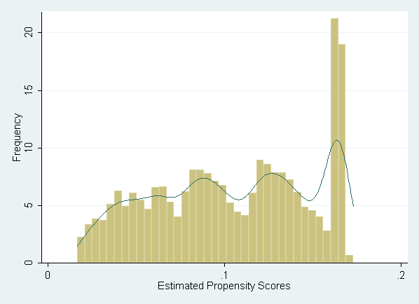
Figure 12.2, Panel A: Full Sample, shown on page 315.
histogram p, kdensity kdenopts(gaussian) xlabel(0(.1).2) ///
	ytitle(Frequency) xtitle(Estimated Propensity Scores)
Summary statistics for the propesnity score variable p, by catholic.
by catholic, sort: sum p, detail

-------------------------------------------------------------------------------------------
-> catholic = no

                        Pr(catholic)
-------------------------------------------------------------
      Percentiles      Smallest
 1%     .0204874       .0164257
 5%     .0304734        .016906
10%     .0398502       .0170297       Obs                5079
25%     .0643826        .017208       Sum of Wgt.        5079

50%     .1018312                      Mean           .1022535
                        Largest       Std. Dev.      .0442736
75%     .1395716       .1729462
90%     .1642913       .1729462       Variance       .0019602
95%     .1647052       .1729462       Skewness      -.1037761
99%     .1652047       .1729462       Kurtosis       1.814756

-------------------------------------------------------------------------------------------
-> catholic = yes

                        Pr(catholic)
-------------------------------------------------------------
      Percentiles      Smallest
 1%     .0311486       .0221945
 5%     .0498571       .0255137
10%      .066539       .0260665       Obs                 592
25%     .0935338       .0266655       Sum of Wgt.         592

50%     .1307598                      Mean            .122727
                        Largest       Std. Dev.      .0377261
75%     .1636715       .1654167
90%     .1645418       .1659938       Variance       .0014233
95%     .1648288       .1668626       Skewness      -.6233737
99%     .1652885       .1729462       Kurtosis       2.378922
Figure 12.2, Panel B: By catholic, shown on page 315.
histogram p, kdensity kdenopts(gaussian) by(catholic, cols(1) legend(off)) ///
	xlabel(0(.1).2) ytitle(Frequency) xtitle(Estimated Propensity Scores)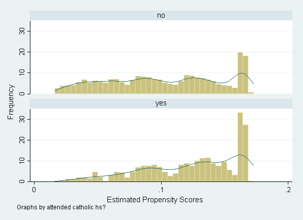
Stratifying on propensity scores, discussed on pages 316-317.
This uses the same set of variables as Model A from Table 12.4. Note that
pscore is a user-written command, and must be downloaded prior to use,
for more information see our FAQ page
How do I use
search to search for programs and additional help?. (Not shown in text.)
pscore catholic inc8 math8 mathfam, logit pscore(p) blockid(b) numblo(5)


****************************************************
Algorithm to estimate the propensity score
****************************************************


The treatment is catholic

   attended |
   catholic |
        hs? |      Freq.     Percent        Cum.
------------+-----------------------------------
         no |      5,079       89.56       89.56
        yes |        592       10.44      100.00
------------+-----------------------------------
      Total |      5,671      100.00


Estimation of the propensity score

Iteration 0:   log likelihood = -1897.6568
Iteration 1:   log likelihood = -1840.7214
Iteration 2:   log likelihood = -1837.6047
Iteration 3:   log likelihood = -1837.5922
Iteration 4:   log likelihood = -1837.5922

Logistic regression                               Number of obs   =       5671
                                                  LR chi2(3)      =     120.13
                                                  Prob > chi2     =     0.0000
Log likelihood = -1837.5922                       Pseudo R2       =     0.0317

------------------------------------------------------------------------------
    catholic |      Coef.   Std. Err.      z    P>|z|     [95% Conf. Interval]
-------------+----------------------------------------------------------------
        inc8 |   .0618026   .0140542     4.40   0.000     .0342569    .0893482
       math8 |   .0429594    .011135     3.86   0.000     .0211352    .0647836
     mathfam |   -.000734   .0002615    -2.81   0.005    -.0012466   -.0002214
       _cons |  -5.208846   .5863848    -8.88   0.000    -6.358139   -4.059553
------------------------------------------------------------------------------


Description of the estimated propensity score

                 Estimated propensity score
-------------------------------------------------------------
      Percentiles      Smallest
 1%     .0300386       .0241574
 5%     .0400463       .0250049
10%     .0488683       .0252239       Obs                5671
25%     .0700201         .02554       Sum of Wgt.        5671

50%     .1023014                      Mean           .1043908
                        Largest       Std. Dev.      .0442227
75%     .1299765       .1898257
90%     .1795338       .1898437       Variance       .0019556
95%     .1835134       .1899649       Skewness       .3693322
99%      .187957       .1900232       Kurtosis       2.215181


******************************************************
Step 1: Identification of the optimal number of blocks
Use option detail if you want more detailed output
******************************************************


The final number of blocks is 4

This number of blocks ensures that the mean propensity score
is not different for treated and controls in each blocks


**********************************************************
Step 2: Test of balancing property of the propensity score
Use option detail if you want more detailed output
**********************************************************

Variable inc8 is not balanced in block 4

Variable mathfam is not balanced in block 4

The balancing property is not satisfied

Try a different specification of the propensity score

  Inferior |
  of block | attended catholic hs?
of pscore  |        no        yes |     Total
-----------+----------------------+----------
         0 |       588         18 |       606
       .05 |     1,002         56 |     1,058
      .075 |     1,010        113 |     1,123
        .1 |     2,479        405 |     2,884
-----------+----------------------+----------
     Total |     5,079        592 |     5,671


*******************************************
End of the algorithm to estimate the pscore
*******************************************
Estimate the propensity score blocks shown in Table 12.5 on page 318.
(Output not shown in text.)
* drop propensity score variables if they already exist
drop p b

pscore catholic inc8 inc8sq math8 mathfam, logit pscore(p) blockid(b) numblo(5)


****************************************************
Algorithm to estimate the propensity score
****************************************************


The treatment is catholic

   attended |
   catholic |
        hs? |      Freq.     Percent        Cum.
------------+-----------------------------------
         no |      5,079       89.56       89.56
        yes |        592       10.44      100.00
------------+-----------------------------------
      Total |      5,671      100.00


Estimation of the propensity score

Iteration 0:   log likelihood = -1897.6568
Iteration 1:   log likelihood = -1838.7904
Iteration 2:   log likelihood = -1833.6223
Iteration 3:   log likelihood = -1833.5413
Iteration 4:   log likelihood = -1833.5413

Logistic regression                               Number of obs   =       5671
                                                  LR chi2(4)      =     128.23
                                                  Prob > chi2     =     0.0000
Log likelihood = -1833.5413                       Pseudo R2       =     0.0338

------------------------------------------------------------------------------
    catholic |      Coef.   Std. Err.      z    P>|z|     [95% Conf. Interval]
-------------+----------------------------------------------------------------
        inc8 |   .0869049    .017354     5.01   0.000     .0528918     .120918
      inc8sq |  -.0004382   .0001569    -2.79   0.005    -.0007458   -.0001306
       math8 |   .0355965   .0119779     2.97   0.003     .0121202    .0590728
     mathfam |  -.0005647   .0002821    -2.00   0.045    -.0011175   -.0000119
       _cons |  -5.362148   .6190447    -8.66   0.000    -6.575453   -4.148842
------------------------------------------------------------------------------


Description of the estimated propensity score

                 Estimated propensity score
-------------------------------------------------------------
      Percentiles      Smallest
 1%     .0208345       .0164257
 5%     .0320812        .016906
10%     .0408223       .0170297       Obs                5671
25%     .0672965        .017208       Sum of Wgt.        5671

50%     .1056115                      Mean           .1043908
                        Largest       Std. Dev.      .0440799
75%      .142168       .1729462
90%     .1643515       .1729462       Variance        .001943
95%     .1647264       .1729462       Skewness      -.1636008
99%     .1652305       .1729462       Kurtosis        1.83253


******************************************************
Step 1: Identification of the optimal number of blocks
Use option detail if you want more detailed output
******************************************************


The final number of blocks is 6

This number of blocks ensures that the mean propensity score
is not different for treated and controls in each blocks


**********************************************************
Step 2: Test of balancing property of the propensity score
Use option detail if you want more detailed output
**********************************************************


The balancing property is satisfied


This table shows the inferior bound, the number of treated
and the number of controls for each block

  Inferior |
  of block | attended catholic hs?
of pscore  |        no        yes |     Total
-----------+----------------------+----------
         0 |       810         31 |       841
       .05 |       741         45 |       786
      .075 |       928        100 |     1,028
        .1 |       786         87 |       873
      .125 |       810        145 |       955
       .15 |     1,004        184 |     1,188
-----------+----------------------+----------
     Total |     5,079        592 |     5,671


*******************************************
End of the algorithm to estimate the pscore
*******************************************
Variable means by block from Table 12.5 on page 318. Note that
for Block 3, the average mathematics achievement for catholic students is
listed as 49.63 in the book, but is 51.56 in the table below. Based on
communication with the authors, this appears to be a typographic error in
the book.
table b catholic, contents(freq mean p mean inc8 mean math8 mean math12)

--------------------------------
Number of |attended catholic hs?
block     |        no        yes
----------+---------------------
        1 |       810         31
          | .03562671   .0397066
          |  8.466666   9.814516
          |  43.16351   44.67839
          |  42.74021   45.34968
          |
        2 |       741         45
          | .06206016  .06352629
          |  18.13968   17.52778
          |  47.44714   49.45711
          |  47.14545   50.21756
          |
        3 |       928        100
          |  .0875975  .08860363
          |  26.64197     26.565
          |  48.80288    49.6273
          |  48.79251      51.56
          |
        4 |       786         87
          |  .1138969  .11401803
          |  33.34605   33.36207
          |  52.61875    52.9077
          |  52.02316   54.26402
          |
        5 |       810        145
          | .13605543  .13692428
          |  40.72839   41.46552
          |  55.15296   54.78959
          |  54.71558   56.54048
          |
        6 |     1,004        184
          | .16283171  .16266777
          |  57.33815   58.36956
          |  58.55379   57.85957
          |  56.95275    57.3175
--------------------------------
Tests for differences in academic achievement by catholic, in each block,
shown in Table 12.5 on page 318. Note that the sign of the differences are reversed, but the magnitude
is the same, and that the error in the mean for block 3 discussed above persists.
by b, sort: ttest math12, by(catholic)

-------------------------------------------------------------------------------------------
-> b = 1

Two-sample t test with equal variances
------------------------------------------------------------------------------
Variable |     Obs        Mean    Std. Err.   Std. Dev.   [95% Conf. Interval]
---------+--------------------------------------------------------------------
      no |     810    42.74021    .2449484    6.971353     42.2594    43.22102
     yes |      31    45.34968    1.310109    7.294381    42.67408    48.02528
---------+--------------------------------------------------------------------
combined |     841     42.8364    .2412525    6.996321    42.36287    43.30993
---------+--------------------------------------------------------------------
    diff |           -2.609468    1.277988               -5.117896   -.1010391
------------------------------------------------------------------------------
    diff = mean(no) - mean(yes)                                   t =  -2.0419
Ho: diff = 0                                     degrees of freedom =      839

    Ha: diff < 0                 Ha: diff != 0                 Ha: diff > 0
 Pr(T < t) = 0.0207         Pr(|T| > |t|) = 0.0415          Pr(T > t) = 0.9793

-------------------------------------------------------------------------------------------
-> b = 2

Two-sample t test with equal variances
------------------------------------------------------------------------------
Variable |     Obs        Mean    Std. Err.   Std. Dev.   [95% Conf. Interval]
---------+--------------------------------------------------------------------
      no |     741    47.14545    .2882466    7.846452    46.57957    47.71133
     yes |      45    50.21756    1.136082    7.621067    47.92793    52.50718
---------+--------------------------------------------------------------------
combined |     786    47.32134    .2804101     7.86149    46.77089    47.87178
---------+--------------------------------------------------------------------
    diff |           -3.072103    1.202757                -5.43311   -.7110971
------------------------------------------------------------------------------
    diff = mean(no) - mean(yes)                                   t =  -2.5542
Ho: diff = 0                                     degrees of freedom =      784

    Ha: diff < 0                 Ha: diff != 0                 Ha: diff > 0
 Pr(T < t) = 0.0054         Pr(|T| > |t|) = 0.0108          Pr(T > t) = 0.9946

-------------------------------------------------------------------------------------------
-> b = 3

Two-sample t test with equal variances
------------------------------------------------------------------------------
Variable |     Obs        Mean    Std. Err.   Std. Dev.   [95% Conf. Interval]
---------+--------------------------------------------------------------------
      no |     928    48.79251    .2754558    8.391235    48.25192     49.3331
     yes |     100       51.56    .8071014    8.071014    49.95854    53.16146
---------+--------------------------------------------------------------------
combined |    1028    49.06172    .2618947    8.396983    48.54781    49.57563
---------+--------------------------------------------------------------------
    diff |           -2.767489    .8799826                -4.49426   -1.040718
------------------------------------------------------------------------------
    diff = mean(no) - mean(yes)                                   t =  -3.1449
Ho: diff = 0                                     degrees of freedom =     1026

    Ha: diff < 0                 Ha: diff != 0                 Ha: diff > 0
 Pr(T < t) = 0.0009         Pr(|T| > |t|) = 0.0017          Pr(T > t) = 0.9991

-------------------------------------------------------------------------------------------
-> b = 4

Two-sample t test with equal variances
------------------------------------------------------------------------------
Variable |     Obs        Mean    Std. Err.   Std. Dev.   [95% Conf. Interval]
---------+--------------------------------------------------------------------
      no |     786    52.02316    .3402795    9.539971    51.35519    52.69112
     yes |      87    54.26402    .9397039    8.764975    52.39595    56.13209
---------+--------------------------------------------------------------------
combined |     873    52.24647    .3210069    9.484653    51.61644    52.87651
---------+--------------------------------------------------------------------
    diff |           -2.240868    1.069585               -4.340133   -.1416024
------------------------------------------------------------------------------
    diff = mean(no) - mean(yes)                                   t =  -2.0951
Ho: diff = 0                                     degrees of freedom =      871

    Ha: diff < 0                 Ha: diff != 0                 Ha: diff > 0
 Pr(T < t) = 0.0182         Pr(|T| > |t|) = 0.0365          Pr(T > t) = 0.9818

-------------------------------------------------------------------------------------------
-> b = 5

Two-sample t test with equal variances
------------------------------------------------------------------------------
Variable |     Obs        Mean    Std. Err.   Std. Dev.   [95% Conf. Interval]
---------+--------------------------------------------------------------------
      no |     810    54.71558    .2588964    7.368319    54.20739    55.22377
     yes |     145    56.54048    .5606502    6.751122    55.43232    57.64865
---------+--------------------------------------------------------------------
combined |     955    54.99266    .2363535     7.30405    54.52883    55.45649
---------+--------------------------------------------------------------------
    diff |           -1.824902    .6563147               -3.112891   -.5369135
------------------------------------------------------------------------------
    diff = mean(no) - mean(yes)                                   t =  -2.7805
Ho: diff = 0                                     degrees of freedom =      953

    Ha: diff < 0                 Ha: diff != 0                 Ha: diff > 0
 Pr(T < t) = 0.0028         Pr(|T| > |t|) = 0.0055          Pr(T > t) = 0.9972

-------------------------------------------------------------------------------------------
-> b = 6

Two-sample t test with equal variances
------------------------------------------------------------------------------
Variable |     Obs        Mean    Std. Err.   Std. Dev.   [95% Conf. Interval]
---------+--------------------------------------------------------------------
      no |    1004    56.95275    .2789432    8.838582    56.40537    57.50013
     yes |     184     57.3175    .6020763    8.166961     56.1296     58.5054
---------+--------------------------------------------------------------------
combined |    1188    57.00924    .2534465    8.735635    56.51199     57.5065
---------+--------------------------------------------------------------------
    diff |           -.3647511    .7007456                -1.73959    1.010088
------------------------------------------------------------------------------
    diff = mean(no) - mean(yes)                                   t =  -0.5205
Ho: diff = 0                                     degrees of freedom =     1186

    Ha: diff < 0                 Ha: diff != 0                 Ha: diff > 0
 Pr(T < t) = 0.3014         Pr(|T| > |t|) = 0.6028          Pr(T > t) = 0.6986
Weighted average ATT shown in Table 12.5 on page 318. Note that
atts is part of the same user-written
package as pscore and that the set seed command was used so that
the results of the bootstrap can be replicated.
set seed 53156
atts math12 catholic, pscore(p) blockid(b) bootstrap

ATT estimation with the Stratification method
Analytical standard errors

---------------------------------------------------------
n. treat.   n. contr.         ATT   Std. Err.           t
---------------------------------------------------------

      592        5079       1.727       0.347       4.975

---------------------------------------------------------


Bootstrapping of standard errors

command:      atts math12 catholic , pscore(p) blockid(b)
statistic:    atts       = r(atts)

Bootstrap statistics                              Number of obs    =      5671
                                                  Replications     =        50

------------------------------------------------------------------------------
Variable     |  Reps  Observed      Bias  Std. Err. [95% Conf. Interval]
-------------+----------------------------------------------------------------
        atts |    50   1.72731  -.044933  .3138169   1.096672   2.357949   (N)
             |                                       1.135532   2.304237   (P)
             |                                       1.273374   2.393047  (BC)
------------------------------------------------------------------------------
Note:  N   = normal
       P   = percentile
       BC  = bias-corrected


ATT estimation with the Stratification method
Bootstrapped standard errors

---------------------------------------------------------
n. treat.   n. contr.         ATT   Std. Err.           t
---------------------------------------------------------

      592        5079       1.727       0.314       5.504

---------------------------------------------------------
The following few examples demonstrate difference methods of
analyzing the same data, treating the propensity scores as an optimal composite
covariate.Method A: Controlling for block by estimating the relationship between math12 and
catholic separately in each
block.
sort b

statsby _b[catholic] e(N), by(b) noisily sav(CathSlopes3,replace): regress math12 catholic

statsby: First call to regress with data as is:

. regress math12 catholic

      Source |       SS       df       MS              Number of obs =    5671
-------------+------------------------------           F(  1,  5669) =   90.48
       Model |   8043.1077     1   8043.1077           Prob > F      =  0.0000
    Residual |  503934.635  5669  88.8930385           R-squared     =  0.0157
-------------+------------------------------           Adj R-squared =  0.0155
       Total |  511977.743  5670  90.2958982           Root MSE      =  9.4283

------------------------------------------------------------------------------
      math12 |      Coef.   Std. Err.      t    P>|t|     [95% Conf. Interval]
-------------+----------------------------------------------------------------
    catholic |    3.89486   .4094621     9.51   0.000     3.092157    4.697562
       _cons |   50.64465   .1322954   382.81   0.000      50.3853      50.904
------------------------------------------------------------------------------

statsby legend:

      command:  regress math12 catholic
      _stat_1:  _b[catholic]
      _stat_2:  e(N)
           by:  b

Statsby groups

running (regress math12 catholic) on group 1

. regress math12 catholic

      Source |       SS       df       MS              Number of obs =     841
-------------+------------------------------           F(  1,   839) =    4.17
       Model |  203.308037     1  203.308037           Prob > F      =  0.0415
    Residual |  40913.4431   839  48.7645329           R-squared     =  0.0049
-------------+------------------------------           Adj R-squared =  0.0038
       Total |  41116.7512   840  48.9485133           Root MSE      =  6.9832

------------------------------------------------------------------------------
      math12 |      Coef.   Std. Err.      t    P>|t|     [95% Conf. Interval]
-------------+----------------------------------------------------------------
    catholic |   2.609468   1.277988     2.04   0.041     .1010391    5.117896
       _cons |   42.74021   .2453633   174.19   0.000     42.25861    43.22181
------------------------------------------------------------------------------

running (regress math12 catholic) on group 2

. regress math12 catholic

      Source |       SS       df       MS              Number of obs =     786
-------------+------------------------------           F(  1,   784) =    6.52
       Model |  400.386878     1  400.386878           Prob > F      =  0.0108
    Residual |  48114.9879   784  61.3711581           R-squared     =  0.0083
-------------+------------------------------           Adj R-squared =  0.0070
       Total |  48515.3748   785  61.8030252           Root MSE      =   7.834

------------------------------------------------------------------------------
      math12 |      Coef.   Std. Err.      t    P>|t|     [95% Conf. Interval]
-------------+----------------------------------------------------------------
    catholic |   3.072103   1.202757     2.55   0.011     .7110971     5.43311
       _cons |   47.14545   .2877882   163.82   0.000     46.58053    47.71038
------------------------------------------------------------------------------

running (regress math12 catholic) on group 3

. regress math12 catholic

      Source |       SS       df       MS              Number of obs =    1028
-------------+------------------------------           F(  1,  1026) =    9.89
       Model |  691.395779     1  691.395779           Prob > F      =  0.0017
    Residual |  71721.6733  1026   69.904165           R-squared     =  0.0095
-------------+------------------------------           Adj R-squared =  0.0086
       Total |   72413.069  1027  70.5093175           Root MSE      =  8.3609

------------------------------------------------------------------------------
      math12 |      Coef.   Std. Err.      t    P>|t|     [95% Conf. Interval]
-------------+----------------------------------------------------------------
    catholic |   2.767489   .8799826     3.14   0.002     1.040718     4.49426
       _cons |   48.79251    .274459   177.78   0.000     48.25395    49.33108
------------------------------------------------------------------------------

running (regress math12 catholic) on group 4

. regress math12 catholic

      Source |       SS       df       MS              Number of obs =     873
-------------+------------------------------           F(  1,   871) =    4.39
       Model |  393.332574     1  393.332574           Prob > F      =  0.0365
    Residual |  78050.6082   871  89.6103423           R-squared     =  0.0050
-------------+------------------------------           Adj R-squared =  0.0039
       Total |  78443.9407   872  89.9586476           Root MSE      =  9.4663

------------------------------------------------------------------------------
      math12 |      Coef.   Std. Err.      t    P>|t|     [95% Conf. Interval]
-------------+----------------------------------------------------------------
    catholic |   2.240868   1.069585     2.10   0.036     .1416024    4.340133
       _cons |   52.02316   .3376508   154.07   0.000     51.36045    52.68586
------------------------------------------------------------------------------

running (regress math12 catholic) on group 5

. regress math12 catholic

      Source |       SS       df       MS              Number of obs =     955
-------------+------------------------------           F(  1,   953) =    7.73
       Model |   409.57076     1   409.57076           Prob > F      =  0.0055
    Residual |  50485.5136   953  52.9753553           R-squared     =  0.0080
-------------+------------------------------           Adj R-squared =  0.0070
       Total |  50895.0844   954  53.3491451           Root MSE      =  7.2784

------------------------------------------------------------------------------
      math12 |      Coef.   Std. Err.      t    P>|t|     [95% Conf. Interval]
-------------+----------------------------------------------------------------
    catholic |   1.824902   .6563147     2.78   0.006     .5369135    3.112891
       _cons |   54.71558   .2557375   213.95   0.000     54.21371    55.21745
------------------------------------------------------------------------------

running (regress math12 catholic) on group 6

. regress math12 catholic

      Source |       SS       df       MS              Number of obs =    1188
-------------+------------------------------           F(  1,  1186) =    0.27
       Model |  20.6884702     1  20.6884702           Prob > F      =  0.6028
    Residual |  90560.8493  1186  76.3582203           R-squared     =  0.0002
-------------+------------------------------           Adj R-squared = -0.0006
       Total |  90581.5377  1187  76.3113208           Root MSE      =  8.7383

------------------------------------------------------------------------------
      math12 |      Coef.   Std. Err.      t    P>|t|     [95% Conf. Interval]
-------------+----------------------------------------------------------------
    catholic |   .3647511   .7007456     0.52   0.603    -1.010088     1.73959
       _cons |   56.95275   .2757789   206.52   0.000     56.41168    57.49382
------------------------------------------------------------------------------
Distribution of coefficients for catholic (predicting math12)
across the propensity score blocks. Note that the syntax shown below is run
from a .do file, the block of syntax should be run all at once. (Not shown
in text.)
preserve
use https://stats.idre.ucla.edu/stat/stata/examples/methods_matter/chapter12/CathSlopes3, clear
list
histogram _stat_1, bin(3) frequency kdensity kdenopts(gaussian)
restore

     +------------------------+
     | b    _stat_1   _stat_2 |
     |------------------------|
  1. | 1   2.609468       841 |
  2. | 2   3.072104       786 |
  3. | 3   2.767489      1028 |
  4. | 4   2.240868       873 |
  5. | 5   1.824902       955 |
     |------------------------|
  6. | 6   .3647511      1188 |
     +------------------------+
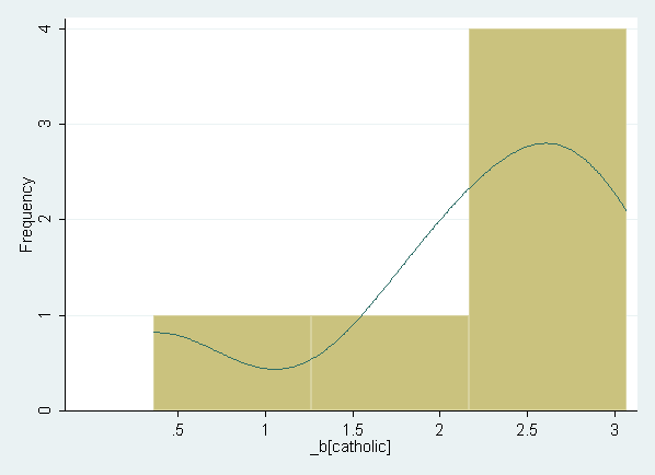
Method B: Estimate the relationship between math12 and catholic in all blocks at the same
time, using fixed effects the blocks. Note that this model includes
the intercept and dummy variables for blocks 2 to 6. (Not shown in text.)
xi:  regress math12 catholic i.b
i.b               _Ib_1-6             (naturally coded; _Ib_1 omitted)

      Source |       SS       df       MS              Number of obs =    5671
-------------+------------------------------           F(  6,  5664) =  326.67
       Model |  131623.108     6  21937.1846           Prob > F      =  0.0000
    Residual |  380354.635  5664  67.1530076           R-squared     =  0.2571
-------------+------------------------------           Adj R-squared =  0.2563
       Total |  511977.743  5670  90.2958982           Root MSE      =  8.1947

------------------------------------------------------------------------------
      math12 |      Coef.   Std. Err.      t    P>|t|     [95% Conf. Interval]
-------------+----------------------------------------------------------------
    catholic |   1.761271   .3595793     4.90   0.000     1.056358    2.466184
       _Ib_2 |   4.449025   .4066192    10.94   0.000     3.651895    5.246154
       _Ib_3 |   6.118917   .3816345    16.03   0.000     5.370767    6.867066
       _Ib_4 |   9.299475   .3965866    23.45   0.000     8.522013    10.07694
       _Ib_5 |   11.95377   .3897119    30.67   0.000     11.18978    12.71775
       _Ib_6 |   13.96498   .3717204    37.57   0.000     13.23626    14.69369
       _cons |   42.77148   .2828863   151.20   0.000     42.21691    43.32604
------------------------------------------------------------------------------
This model can also be estimated using the factor variable syntax introduced
in Stata 11. (Not shown in text.)
regress math12 catholic i.b

      Source |       SS       df       MS              Number of obs =    5671
-------------+------------------------------           F(  6,  5664) =  326.67
       Model |  131623.108     6  21937.1846           Prob > F      =  0.0000
    Residual |  380354.635  5664  67.1530076           R-squared     =  0.2571
-------------+------------------------------           Adj R-squared =  0.2563
       Total |  511977.743  5670  90.2958982           Root MSE      =  8.1947

------------------------------------------------------------------------------
      math12 |      Coef.   Std. Err.      t    P>|t|     [95% Conf. Interval]
-------------+----------------------------------------------------------------
    catholic |   1.761271   .3595793     4.90   0.000     1.056358    2.466184
             |
           b |
          2  |   4.449025   .4066192    10.94   0.000     3.651895    5.246154
          3  |   6.118917   .3816345    16.03   0.000     5.370767    6.867066
          4  |   9.299475   .3965866    23.45   0.000     8.522013    10.07694
          5  |   11.95377   .3897119    30.67   0.000     11.18978    12.71775
          6  |   13.96498   .3717204    37.57   0.000     13.23626    14.69369
             |
       _cons |   42.77148   .2828863   151.20   0.000     42.21691    43.32604
------------------------------------------------------------------------------
An equivalent model with no intercept and a fixed effect for each block.
(Not shown in text.)
xi i.b, noomit
regress math12 catholic _Ib_1-_Ib_6, noconstant

      Source |       SS       df       MS              Number of obs =    5671
-------------+------------------------------           F(  7,  5664) =31721.90
       Model |  14911547.1     7  2130221.02           Prob > F      =  0.0000
    Residual |  380354.635  5664  67.1530076           R-squared     =  0.9751
-------------+------------------------------           Adj R-squared =  0.9751
       Total |  15291901.8  5671  2696.50887           Root MSE      =  8.1947

------------------------------------------------------------------------------
      math12 |      Coef.   Std. Err.      t    P>|t|     [95% Conf. Interval]
-------------+----------------------------------------------------------------
    catholic |   1.761271   .3595793     4.90   0.000     1.056358    2.466184
       _Ib_1 |   42.77148   .2828863   151.20   0.000     42.21691    43.32604
       _Ib_2 |    47.2205   .2930191   161.15   0.000     46.64607    47.79493
       _Ib_3 |   48.89039   .2579679   189.52   0.000     48.38468    49.39611
       _Ib_4 |   52.07095   .2796537   186.20   0.000     51.52272    52.61918
       _Ib_5 |   54.72524    .270736   202.14   0.000      54.1945    55.25599
       _Ib_6 |   56.73645   .2441879   232.35   0.000     56.25775    57.21515
------------------------------------------------------------------------------
This model can also be estimated using the factor variable syntax introduced
in Stata 11. Note that the dummy variables do not need to be created using xi.
regress math12 catholic ibn.b, noconstant

      Source |       SS       df       MS              Number of obs =    5671
-------------+------------------------------           F(  7,  5664) =31721.90
       Model |  14911547.1     7  2130221.02           Prob > F      =  0.0000
    Residual |  380354.635  5664  67.1530076           R-squared     =  0.9751
-------------+------------------------------           Adj R-squared =  0.9751
       Total |  15291901.8  5671  2696.50887           Root MSE      =  8.1947

------------------------------------------------------------------------------
      math12 |      Coef.   Std. Err.      t    P>|t|     [95% Conf. Interval]
-------------+----------------------------------------------------------------
    catholic |   1.761271   .3595793     4.90   0.000     1.056358    2.466184
             |
           b |
          1  |   42.77148   .2828863   151.20   0.000     42.21691    43.32604
          2  |    47.2205   .2930191   161.15   0.000     46.64607    47.79493
          3  |   48.89039   .2579679   189.52   0.000     48.38468    49.39611
          4  |   52.07095   .2796537   186.20   0.000     51.52272    52.61918
          5  |   54.72524    .270736   202.14   0.000      54.1945    55.25599
          6  |   56.73645   .2441879   232.35   0.000     56.25775    57.21515
------------------------------------------------------------------------------
Method C: Controlling for propensities (as a linear effect). (Not shown in text.)
regress math12 catholic p

      Source |       SS       df       MS              Number of obs =    5671
-------------+------------------------------           F(  2,  5668) =  996.64
       Model |  133204.471     2  66602.2355           Prob > F      =  0.0000
    Residual |  378773.272  5668  66.8266182           R-squared     =  0.2602
-------------+------------------------------           Adj R-squared =  0.2599
       Total |  511977.743  5670  90.2958982           Root MSE      =  8.1748

------------------------------------------------------------------------------
      math12 |      Coef.   Std. Err.      t    P>|t|     [95% Conf. Interval]
-------------+----------------------------------------------------------------
    catholic |   1.690306   .3586574     4.71   0.000        .9872    2.393411
           p |   107.6782   2.488099    43.28   0.000     102.8006    112.5559
       _cons |   39.63417   .2790795   142.02   0.000     39.08707    40.18127
------------------------------------------------------------------------------
Create propensity score blocks for Table 12.6 on page 320. (Output not shown
in text.)
* drop p and b from previous examples
drop p b

pscore catholic inc8 inc8sq math8 mathfam fhowfar mhowfar fight8 nohw8 ///
	disrupt8 riskdrop8, logit pscore(p) blockid(b) numblo(10)

****************************************************
Algorithm to estimate the propensity score
****************************************************


The treatment is catholic

   attended |
   catholic |
        hs? |      Freq.     Percent        Cum.
------------+-----------------------------------
         no |      5,079       89.56       89.56
        yes |        592       10.44      100.00
------------+-----------------------------------
      Total |      5,671      100.00


Estimation of the propensity score

Iteration 0:   log likelihood = -1897.6568
Iteration 1:   log likelihood = -1814.3485
Iteration 2:   log likelihood = -1804.4342
Iteration 3:   log likelihood = -1804.1259
Iteration 4:   log likelihood = -1804.1254

Logistic regression                               Number of obs   =       5671
                                                  LR chi2(10)     =     187.06
                                                  Prob > chi2     =     0.0000
Log likelihood = -1804.1254                       Pseudo R2       =     0.0493

------------------------------------------------------------------------------
    catholic |      Coef.   Std. Err.      z    P>|z|     [95% Conf. Interval]
-------------+----------------------------------------------------------------
        inc8 |   .0544244   .0190915     2.85   0.004     .0170058     .091843
      inc8sq |  -.0001894   .0001732    -1.09   0.274     -.000529    .0001501
       math8 |   .0215572   .0123655     1.74   0.081    -.0026787    .0457932
     mathfam |  -.0004537   .0002873    -1.58   0.114    -.0010169    .0001095
     fhowfar |   .1963326   .0866025     2.27   0.023     .0265949    .3660703
     mhowfar |   .0256765    .086921     0.30   0.768    -.1446855    .1960384
      fight8 |  -.4742975   .3246254    -1.46   0.144    -1.110552    .1619566
       nohw8 |  -.6880268   .1760058    -3.91   0.000    -1.032992   -.3430618
    disrupt8 |   .6927506   .3858711     1.80   0.073    -.0635429    1.449044
   riskdrop8 |  -.3033031   .0843134    -3.60   0.000    -.4685543   -.1380518
       _cons |  -4.981792    .703233    -7.08   0.000    -6.360104   -3.603481
------------------------------------------------------------------------------


Description of the estimated propensity score

                 Estimated propensity score
-------------------------------------------------------------
      Percentiles      Smallest
 1%     .0108842       .0025956
 5%     .0204415       .0032377
10%     .0313083       .0036331       Obs                5671
25%     .0595311       .0047923       Sum of Wgt.        5671

50%     .1072919                      Mean           .1043908
                        Largest       Std. Dev.      .0530622
75%     .1453336       .2551539
90%     .1744188       .2571622       Variance       .0028156
95%     .1858031       .2619453       Skewness       .0612084
99%     .2138622        .262511       Kurtosis       2.084156


******************************************************
Step 1: Identification of the optimal number of blocks
Use option detail if you want more detailed output
******************************************************


The final number of blocks is 5

This number of blocks ensures that the mean propensity score
is not different for treated and controls in each blocks


**********************************************************
Step 2: Test of balancing property of the propensity score
Use option detail if you want more detailed output
**********************************************************


The balancing property is satisfied


This table shows the inferior bound, the number of treated
and the number of controls for each block

  Inferior |
  of block | attended catholic hs?
of pscore  |        no        yes |     Total
-----------+----------------------+----------
         0 |     1,089         34 |     1,123
       .05 |     1,431        110 |     1,541
        .1 |     1,599        253 |     1,852
       .15 |       829        160 |       989
        .2 |       131         35 |       166
-----------+----------------------+----------
     Total |     5,079        592 |     5,671


*******************************************
End of the algorithm to estimate the pscore
*******************************************
Distribution of estimated propensity scores based on the model for
Table 12.6. (Not shown in text.)
sum p, detail

                 Estimated propensity score
-------------------------------------------------------------
      Percentiles      Smallest
 1%     .0108842       .0025956
 5%     .0204415       .0032377
10%     .0313083       .0036331       Obs                5671
25%     .0595311       .0047923       Sum of Wgt.        5671

50%     .1072919                      Mean           .1043908
                        Largest       Std. Dev.      .0530622
75%     .1453336       .2551539
90%     .1744188       .2571622       Variance       .0028156
95%     .1858031       .2619453       Skewness       .0612084
99%     .2138622        .262511       Kurtosis       2.084156


histogram p, kdensity kdenopts(gaussian) xlabel(0(.1).3) ///
	ytitle(Frequency) xtitle(Estimated Propensity Scores)
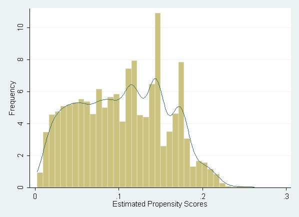
Distribution of propensity scores by catholic.
by catholic, sort: sum p, detail

-------------------------------------------------------------------------------------------
-> catholic = no

                 Estimated propensity score
-------------------------------------------------------------
      Percentiles      Smallest
 1%     .0104881       .0025956
 5%     .0195553       .0032377
10%     .0297857       .0036331       Obs                5079
25%     .0565767       .0047923       Sum of Wgt.        5079

50%     .1008954                      Mean           .1012761
                        Largest       Std. Dev.      .0529831
75%     .1440137       .2551539
90%      .173256       .2571622       Variance       .0028072
95%     .1824525       .2619453       Skewness       .1216262
99%     .2133106        .262511       Kurtosis       2.085038

-------------------------------------------------------------------------------------------
-> catholic = yes

                 Estimated propensity score
-------------------------------------------------------------
      Percentiles      Smallest
 1%     .0229674       .0099903
 5%     .0470903        .011172
10%     .0699177        .018644       Obs                 592
25%     .1003173       .0196516       Sum of Wgt.         592

50%     .1355502                      Mean           .1311124
                        Largest       Std. Dev.      .0457582
75%      .169457       .2266057
90%     .1842547        .228063       Variance       .0020938
95%     .2031689       .2391276       Skewness      -.3031523
99%     .2224912       .2462637       Kurtosis       2.624687


histogram p, kdensity kdenopts(gaussian) by(catholic, cols(1) legend(off)) ///
	xlabel(0(.1).3) ytitle(Frequency) xtitle(Estimated Propensity Scores)
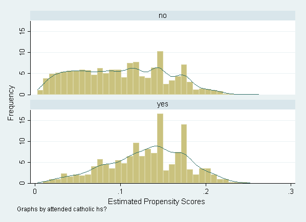
Descriptive statistics for Table 12.6 on page 320.
table b catholic, contents(freq mean p mean math12)

--------------------------------
Number of |attended catholic hs?
block     |        no        yes
----------+---------------------
        1 |     1,089         34
          | .03032015  .03453844
          |  43.66365   46.01353
          |
        2 |     1,431        110
          | .07522784  .07848568
          |  48.85303   51.00237
          |
        3 |     1,599        253
          |  .1270797  .12911088
          |  53.62299   55.38316
          |
        4 |       829        160
          | .17195554  .17329525
          |  56.86899   57.34556
          |
        5 |       131         35
          | .21343681  .21195736
          |  52.50557   55.01257
--------------------------------
Tests for differences in academic achievement by catholic, in each block,
shown in Table 12.6 on page 318. Note that the sign of the differences are reversed, but
the magnitude is the same.
by b, sort: ttest math12, by(catholic)

-------------------------------------------------------------------------------------------
-> b = 1

Two-sample t test with equal variances
------------------------------------------------------------------------------
Variable |     Obs        Mean    Std. Err.   Std. Dev.   [95% Conf. Interval]
---------+--------------------------------------------------------------------
      no |    1089    43.66365    .2303222    7.600632    43.21172    44.11557
     yes |      34    46.01353    1.288496    7.513157    43.39206    48.63499
---------+--------------------------------------------------------------------
combined |    1123    43.73479    .2269499     7.60536     43.2895    44.18008
---------+--------------------------------------------------------------------
    diff |           -2.349884    1.323244               -4.946197    .2464296
------------------------------------------------------------------------------
    diff = mean(no) - mean(yes)                                   t =  -1.7759
Ho: diff = 0                                     degrees of freedom =     1121

    Ha: diff < 0                 Ha: diff != 0                 Ha: diff > 0
 Pr(T < t) = 0.0380         Pr(|T| > |t|) = 0.0760          Pr(T > t) = 0.9620

-------------------------------------------------------------------------------------------
-> b = 2

Two-sample t test with equal variances
------------------------------------------------------------------------------
Variable |     Obs        Mean    Std. Err.   Std. Dev.   [95% Conf. Interval]
---------+--------------------------------------------------------------------
      no |    1431    48.85303    .2310661    8.740896    48.39977     49.3063
     yes |     110    51.00236    .7979284    8.368744     49.4209    52.58383
---------+--------------------------------------------------------------------
combined |    1541    49.00646    .2223837    8.729799    48.57025    49.44266
---------+--------------------------------------------------------------------
    diff |           -2.149331    .8622945               -3.840727   -.4579344
------------------------------------------------------------------------------
    diff = mean(no) - mean(yes)                                   t =  -2.4926
Ho: diff = 0                                     degrees of freedom =     1539

    Ha: diff < 0                 Ha: diff != 0                 Ha: diff > 0
 Pr(T < t) = 0.0064         Pr(|T| > |t|) = 0.0128          Pr(T > t) = 0.9936

-------------------------------------------------------------------------------------------
-> b = 3

Two-sample t test with equal variances
------------------------------------------------------------------------------
Variable |     Obs        Mean    Std. Err.   Std. Dev.   [95% Conf. Interval]
---------+--------------------------------------------------------------------
      no |    1599    53.62299    .2155456     8.61913    53.20021    54.04577
     yes |     253    55.38316    .5098506     8.10967    54.37905    56.38727
---------+--------------------------------------------------------------------
combined |    1852    53.86344     .199154    8.570566    53.47285    54.25403
---------+--------------------------------------------------------------------
    diff |           -1.760173    .5786011               -2.894952   -.6253928
------------------------------------------------------------------------------
    diff = mean(no) - mean(yes)                                   t =  -3.0421
Ho: diff = 0                                     degrees of freedom =     1850

    Ha: diff < 0                 Ha: diff != 0                 Ha: diff > 0
 Pr(T < t) = 0.0012         Pr(|T| > |t|) = 0.0024          Pr(T > t) = 0.9988

-------------------------------------------------------------------------------------------
-> b = 4

Two-sample t test with equal variances
------------------------------------------------------------------------------
Variable |     Obs        Mean    Std. Err.   Std. Dev.   [95% Conf. Interval]
---------+--------------------------------------------------------------------
      no |     829    56.86899    .2909555    8.377295    56.29789    57.44008
     yes |     160    57.34556    .5922284    7.491162    56.17591    58.51521
---------+--------------------------------------------------------------------
combined |     989    56.94609    .2619749    8.238684      56.432    57.46018
---------+--------------------------------------------------------------------
    diff |           -.4765759    .7116066               -1.873012    .9198599
------------------------------------------------------------------------------
    diff = mean(no) - mean(yes)                                   t =  -0.6697
Ho: diff = 0                                     degrees of freedom =      987

    Ha: diff < 0                 Ha: diff != 0                 Ha: diff > 0
 Pr(T < t) = 0.2516         Pr(|T| > |t|) = 0.5032          Pr(T > t) = 0.7484

-------------------------------------------------------------------------------------------
-> b = 5

Two-sample t test with equal variances
------------------------------------------------------------------------------
Variable |     Obs        Mean    Std. Err.   Std. Dev.   [95% Conf. Interval]
---------+--------------------------------------------------------------------
      no |     131    52.50557    .6960753    7.966946    51.12847    53.88267
     yes |      35    55.01257    1.310023    7.750203    52.35028    57.67486
---------+--------------------------------------------------------------------
combined |     166    53.03416    .6181866    7.964777    51.81358    54.25473
---------+--------------------------------------------------------------------
    diff |           -2.506999    1.507463               -5.483536    .4695381
------------------------------------------------------------------------------
    diff = mean(no) - mean(yes)                                   t =  -1.6631
Ho: diff = 0                                     degrees of freedom =      164

    Ha: diff < 0                 Ha: diff != 0                 Ha: diff > 0
 Pr(T < t) = 0.0491         Pr(|T| > |t|) = 0.0982          Pr(T > t) = 0.9509
ATT shown in Table 12.6 on page 320.
set seed 7492
atts math12 catholic, pscore(p) blockid(b) bootstrap


ATT estimation with the Stratification method
Analytical standard errors

---------------------------------------------------------
n. treat.   n. contr.         ATT   Std. Err.           t
---------------------------------------------------------

      592        5079       1.564       0.353       4.424

---------------------------------------------------------


Bootstrapping of standard errors

command:      atts math12 catholic , pscore(p) blockid(b)
statistic:    atts       = r(atts)

Bootstrap statistics                              Number of obs    =      5671
                                                  Replications     =        50

------------------------------------------------------------------------------
Variable     |  Reps  Observed      Bias  Std. Err. [95% Conf. Interval]
-------------+----------------------------------------------------------------
        atts |    50  1.563586  .0258251  .3812768   .7973821   2.329791   (N)
             |                                       .7701139   2.242676   (P)
             |                                        .605822   2.242676  (BC)
------------------------------------------------------------------------------
Note:  N   = normal
       P   = percentile
       BC  = bias-corrected


ATT estimation with the Stratification method
Bootstrapped standard errors

---------------------------------------------------------
n. treat.   n. contr.         ATT   Std. Err.           t
---------------------------------------------------------

      592        5079       1.564       0.381       4.101

---------------------------------------------------------
Additional methods of controlling for propensity scores, using the model
with additional covariates used to estimate propensity (i.e. using the propensity model
from Table 12.6).
Method A: Controlling for block by estimating the relationship between math12 and
catholic separately in each block.
sort b
statsby _b[catholic] e(N), by(b) noisily sav(Cathslopes4,replace): regress math12 catholic

statsby: First call to regress with data as is:

. regress math12 catholic

      Source |       SS       df       MS              Number of obs =    5671
-------------+------------------------------           F(  1,  5669) =   90.48
       Model |   8043.1077     1   8043.1077           Prob > F      =  0.0000
    Residual |  503934.635  5669  88.8930385           R-squared     =  0.0157
-------------+------------------------------           Adj R-squared =  0.0155
       Total |  511977.743  5670  90.2958982           Root MSE      =  9.4283

------------------------------------------------------------------------------
      math12 |      Coef.   Std. Err.      t    P>|t|     [95% Conf. Interval]
-------------+----------------------------------------------------------------
    catholic |    3.89486   .4094621     9.51   0.000     3.092157    4.697562
       _cons |   50.64465   .1322954   382.81   0.000      50.3853      50.904
------------------------------------------------------------------------------

statsby legend:

      command:  regress math12 catholic
      _stat_1:  _b[catholic]
      _stat_2:  e(N)
           by:  b

Statsby groups

running (regress math12 catholic) on group 1

. regress math12 catholic

      Source |       SS       df       MS              Number of obs =    1123
-------------+------------------------------           F(  1,  1121) =    3.15
       Model |  182.062217     1  182.062217           Prob > F      =  0.0760
    Residual |  64716.1076  1121  57.7306936           R-squared     =  0.0028
-------------+------------------------------           Adj R-squared =  0.0019
       Total |  64898.1698  1122  57.8415061           Root MSE      =  7.5981

------------------------------------------------------------------------------
      math12 |      Coef.   Std. Err.      t    P>|t|     [95% Conf. Interval]
-------------+----------------------------------------------------------------
    catholic |   2.349884   1.323244     1.78   0.076    -.2464296    4.946197
       _cons |   43.66365   .2302446   189.64   0.000     43.21189     44.1154
------------------------------------------------------------------------------

running (regress math12 catholic) on group 2

. regress math12 catholic

      Source |       SS       df       MS              Number of obs =    1541
-------------+------------------------------           F(  1,  1539) =    6.21
       Model |  471.884989     1  471.884989           Prob > F      =  0.0128
    Residual |   116890.58  1539  75.9522939           R-squared     =  0.0040
-------------+------------------------------           Adj R-squared =  0.0034
       Total |  117362.465  1540  76.2093931           Root MSE      =  8.7151

------------------------------------------------------------------------------
      math12 |      Coef.   Std. Err.      t    P>|t|     [95% Conf. Interval]
-------------+----------------------------------------------------------------
    catholic |   2.149331   .8622945     2.49   0.013     .4579344    3.840727
       _cons |   48.85303   .2303831   212.05   0.000     48.40113    49.30493
------------------------------------------------------------------------------

running (regress math12 catholic) on group 3

. regress math12 catholic

      Source |       SS       df       MS              Number of obs =    1852
-------------+------------------------------           F(  1,  1850) =    9.25
       Model |  676.765989     1  676.765989           Prob > F      =  0.0024
    Residual |  135287.688  1850  73.1284801           R-squared     =  0.0050
-------------+------------------------------           Adj R-squared =  0.0044
       Total |  135964.454  1851  73.4545944           Root MSE      =  8.5515

------------------------------------------------------------------------------
      math12 |      Coef.   Std. Err.      t    P>|t|     [95% Conf. Interval]
-------------+----------------------------------------------------------------
    catholic |   1.760173   .5786011     3.04   0.002     .6253928    2.894952
       _cons |   53.62299   .2138548   250.74   0.000     53.20357    54.04241
------------------------------------------------------------------------------

running (regress math12 catholic) on group 4

. regress math12 catholic

      Source |       SS       df       MS              Number of obs =     989
-------------+------------------------------           F(  1,   987) =    0.45
       Model |  30.4608727     1  30.4608727           Prob > F      =  0.5032
    Residual |   67030.949   987  67.9138288           R-squared     =  0.0005
-------------+------------------------------           Adj R-squared = -0.0006
       Total |  67061.4099   988   67.875921           Root MSE      =   8.241

------------------------------------------------------------------------------
      math12 |      Coef.   Std. Err.      t    P>|t|     [95% Conf. Interval]
-------------+----------------------------------------------------------------
    catholic |   .4765759   .7116066     0.67   0.503    -.9198599    1.873012
       _cons |   56.86899   .2862212   198.69   0.000     56.30731    57.43066
------------------------------------------------------------------------------

running (regress math12 catholic) on group 5

. regress math12 catholic

      Source |       SS       df       MS              Number of obs =     166
-------------+------------------------------           F(  1,   164) =    2.77
       Model |  173.595927     1  173.595927           Prob > F      =  0.0982
    Residual |  10293.6209   164  62.7659812           R-squared     =  0.0166
-------------+------------------------------           Adj R-squared =  0.0106
       Total |  10467.2168   165  63.4376779           Root MSE      =  7.9225

------------------------------------------------------------------------------
      math12 |      Coef.   Std. Err.      t    P>|t|     [95% Conf. Interval]
-------------+----------------------------------------------------------------
    catholic |   2.506999   1.507463     1.66   0.098    -.4695381    5.483536
       _cons |   52.50557   .6921919    75.85   0.000     51.13882    53.87233
------------------------------------------------------------------------------
Distribution of coefficients for catholic (predicting math12) across
the propensity score blocks. Note that the syntax shown below is run from a .do file,
the block of syntax should be run all at once. (Not shown in text.)
preserve
use https://stats.idre.ucla.edu/stat/stata/examples/methods_matter/chapter12/CathSlopes4, clear
list
histogram _stat_1, bin(3) frequency kdensity kdenopts(gaussian)
restore

     +------------------------+
     | b    _stat_1   _stat_2 |
     |------------------------|
  1. | 1   2.349884      1123 |
  2. | 2   2.149331      1541 |
  3. | 3   1.760173      1852 |
  4. | 4   .4765759       989 |
  5. | 5   2.506999       166 |
     +------------------------+
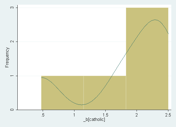
Method B: Estimate the relationship between math12 and catholic in all blocks at
the same time, using fixed effects the blocks. Note that this model includes the intercept and
dummy variables for blocks 2 to 6. (Not shown in text.)
xi: regress math12 catholic i.b
i.b               _Ib_1-5             (naturally coded; _Ib_1 omitted)

      Source |       SS       df       MS              Number of obs =    5671
-------------+------------------------------           F(  5,  5665) =  337.52
       Model |  117512.027     5  23502.4055           Prob > F      =  0.0000
    Residual |  394465.715  5665  69.6320768           R-squared     =  0.2295
-------------+------------------------------           Adj R-squared =  0.2288
       Total |  511977.743  5670  90.2958982           Root MSE      =  8.3446

------------------------------------------------------------------------------
      math12 |      Coef.   Std. Err.      t    P>|t|     [95% Conf. Interval]
-------------+----------------------------------------------------------------
    catholic |   1.580998    .367602     4.30   0.000     .8603572    2.301639
       _Ib_2 |   5.206677     .32775    15.89   0.000     4.564162    5.849193
       _Ib_3 |   9.960542    .318012    31.32   0.000     9.337117    10.58397
       _Ib_4 |   13.00339   .3670815    35.42   0.000     12.28377    13.72301
       _Ib_5 |   9.013889   .6970521    12.93   0.000       7.6474    10.38038
       _cons |   43.68692   .2492575   175.27   0.000     43.19828    44.17556
------------------------------------------------------------------------------
This model can also be estimated using the factor variable syntax
introduced in Stata 11. (Not shown in text.)
regress math12 catholic i.b

      Source |       SS       df       MS              Number of obs =    5671
-------------+------------------------------           F(  5,  5665) =  337.52
       Model |  117512.027     5  23502.4055           Prob > F      =  0.0000
    Residual |  394465.715  5665  69.6320768           R-squared     =  0.2295
-------------+------------------------------           Adj R-squared =  0.2288
       Total |  511977.743  5670  90.2958982           Root MSE      =  8.3446

------------------------------------------------------------------------------
      math12 |      Coef.   Std. Err.      t    P>|t|     [95% Conf. Interval]
-------------+----------------------------------------------------------------
    catholic |   1.580998    .367602     4.30   0.000     .8603572    2.301639
             |
           b |
          2  |   5.206677     .32775    15.89   0.000     4.564162    5.849193
          3  |   9.960542    .318012    31.32   0.000     9.337117    10.58397
          4  |   13.00339   .3670815    35.42   0.000     12.28377    13.72301
          5  |   9.013889   .6970521    12.93   0.000       7.6474    10.38038
             |
       _cons |   43.68692   .2492575   175.27   0.000     43.19828    44.17556
------------------------------------------------------------------------------
An equivalent model with no intercept and a fixed effect for each block.
(Not shown in text.)
xi i.b, noomit
regress math12 catholic _Ib_1-_Ib_5, noconstant

      Source |       SS       df       MS              Number of obs =    5671
-------------+------------------------------           F(  6,  5665) =35657.50
       Model |  14897436.1     6  2482906.01           Prob > F      =  0.0000
    Residual |  394465.715  5665  69.6320768           R-squared     =  0.9742
-------------+------------------------------           Adj R-squared =  0.9742
       Total |  15291901.8  5671  2696.50887           Root MSE      =  8.3446

------------------------------------------------------------------------------
      math12 |      Coef.   Std. Err.      t    P>|t|     [95% Conf. Interval]
-------------+----------------------------------------------------------------
    catholic |   1.580998    .367602     4.30   0.000     .8603572    2.301639
       _Ib_1 |   43.68692   .2492575   175.27   0.000     43.19828    44.17556
       _Ib_2 |    48.8936   .2141841   228.28   0.000     48.47372    49.31348
       _Ib_3 |   53.64747   .2003001   267.84   0.000      53.2548    54.04013
       _Ib_4 |   56.69031   .2719252   208.48   0.000     56.15724    57.22339
       _Ib_5 |   52.70081   .6522864    80.79   0.000     51.42208    53.97954
------------------------------------------------------------------------------
This model can also be estimated using the factor variable syntax introduced in Stata 11. Note that the dummy variables do not need to be created using xi.
regress math12 catholic ibn.b, noconstant

      Source |       SS       df       MS              Number of obs =    5671
-------------+------------------------------           F(  6,  5665) =35657.50
       Model |  14897436.1     6  2482906.01           Prob > F      =  0.0000
    Residual |  394465.715  5665  69.6320768           R-squared     =  0.9742
-------------+------------------------------           Adj R-squared =  0.9742
       Total |  15291901.8  5671  2696.50887           Root MSE      =  8.3446

------------------------------------------------------------------------------
      math12 |      Coef.   Std. Err.      t    P>|t|     [95% Conf. Interval]
-------------+----------------------------------------------------------------
    catholic |   1.580998    .367602     4.30   0.000     .8603572    2.301639
             |
           b |
          1  |   43.68692   .2492575   175.27   0.000     43.19828    44.17556
          2  |    48.8936   .2141841   228.28   0.000     48.47372    49.31348
          3  |   53.64747   .2003001   267.84   0.000      53.2548    54.04013
          4  |   56.69031   .2719252   208.48   0.000     56.15724    57.22339
          5  |   52.70081   .6522864    80.79   0.000     51.42208    53.97954
------------------------------------------------------------------------------
Method C: Controlling for propensities (as a linear effect). (Not shown in text.)
regress math12 catholic p

      Source |       SS       df       MS              Number of obs =    5671
-------------+------------------------------           F(  2,  5668) =  802.96
       Model |   113033.68     2  56516.8401           Prob > F      =  0.0000
    Residual |  398944.063  5668  70.3853321           R-squared     =  0.2208
-------------+------------------------------           Adj R-squared =  0.2205
       Total |  511977.743  5670  90.2958982           Root MSE      =  8.3896

------------------------------------------------------------------------------
      math12 |      Coef.   Std. Err.      t    P>|t|     [95% Conf. Interval]
-------------+----------------------------------------------------------------
    catholic |   1.438686   .3698603     3.89   0.000     .7136181    2.163753
           p |   82.32179   2.131477    38.62   0.000     78.14328     86.5003
       _cons |   42.30742   .2458801   172.07   0.000      41.8254    42.78944
------------------------------------------------------------------------------
Controlling for selection using nearest-neighbor matching (with
random draws).
Discussed on page 323. The command attnd is part of the same user-written
package as pscore and atts.
attnd math12 catholic, pscore(p) comsup detail matchvar(neighbor) matchdta(pickdat3) id(id)


****************************************************************
Estimation of the ATT with the nearest neighbor matching method
Random draw version
****************************************************************


 Note: the common support option has been selected
 The region of common support is [.00999032, .24626373]


 The outcome is math12

    Variable |       Obs        Mean    Std. Dev.       Min        Max
-------------+--------------------------------------------------------
      math12 |      5617    51.14784    9.475516      29.88      71.37


 The treatment is catholic

   attended |
   catholic |
        hs? |      Freq.     Percent        Cum.
------------+-----------------------------------
         no |      5,025       89.46       89.46
        yes |        592       10.54      100.00
------------+-----------------------------------
      Total |      5,617      100.00


 The distribution of the pscore is

                 Estimated propensity score
-------------------------------------------------------------
      Percentiles      Smallest
 1%     .0133107       .0099903
 5%     .0224748       .0100709
10%     .0323934       .0101176       Obs                5617
25%     .0604995       .0102946       Sum of Wgt.        5617

50%      .107828                      Mean           .1049281
                        Largest       Std. Dev.      .0522626
75%      .145359       .2322851
90%     .1742154       .2384602       Variance       .0027314
95%     .1851969       .2391276       Skewness       .0475229
99%     .2127406       .2462637       Kurtosis       2.030977


 The program is searching the nearest neighbor of each treated unit.
 This operation may take a while.

 ****************************************************
 Forward search


 ****************************************************
 Backward search


 ****************************************************
 Choice between backward or forward match


****************************************************
Display of final results
****************************************************


The number of treated is
  592


The number of treated which have been matched is
  592


Average absolute pscore difference between treated and controls

    Variable |       Obs        Mean    Std. Dev.       Min        Max
-------------+--------------------------------------------------------
       PSDIF |       592    .0000432    .0003268          0   .0078036


Average outcome of the matched treated

    Variable |       Obs        Mean    Std. Dev.       Min        Max
-------------+--------------------------------------------------------
      math12 |       592    54.53951    8.463153      32.92      71.08


Average outcome of the matched controls

    Variable |     Obs      Weight        Mean   Std. Dev.       Min        Max
-------------+-----------------------------------------------------------------
      math12 |     553         592    53.61822   8.913623      32.05      70.79
(553 real changes made)
(592 real changes made)


ATT estimation with Nearest Neighbor Matching method
(random draw version)
Analytical standard errors

---------------------------------------------------------
n. treat.   n. contr.         ATT    Std. Err.          t
---------------------------------------------------------

      592         553       0.921        0.537      1.716

---------------------------------------------------------
Note: the numbers of treated and controls refer to actual
nearest neighbour matches


*****************************************************************************
End of the estimation with the nearest neighbor matching (random draw) method
*****************************************************************************
Inspect the neighbors based on the above model and estimate ATE.
Note that the syntax shown below is run from a .do file, the block of syntax should
be run all at once. The syntax is shown twice, once as a single block, then with
the output. (Discussed on page 323.)
* Syntax alone
preserve
 use https://stats.idre.ucla.edu/stat/stata/examples/methods_matter/chapter12/pickdat3, clear
 merge id using "https://stats.idre.ucla.edu/stat/stata/examples/methods_matter/chapter12/catholic.dta" , ///
 	unique update
 sort p catholic
 list id p catholic faminc8 math8 fhowfar mhowfar fight8 nohw8 disrupt8 riskdrop8 ///
 	if p<.012 & neighbor==1
 * Estimate ATE directly
 ttest math12 if neighbor==1, by(catholic)
restore


* Syntax with output
preserve
use https://stats.idre.ucla.edu/stat/stata/examples/methods_matter/chapter12/pickdat3, clear
merge id using "https://stats.idre.ucla.edu/stat/stata/examples/methods_matter/chapter12/catholic.dta" , ///
	unique update
id was float now double

sort p catholic
list id p catholic faminc8 math8 fhowfar mhowfar fight8 nohw8 disrupt8 riskdrop8 ///
	if p<.012 & neighbor==1

      +----------------------------------------------------------------------------------+
   1. |      id |        p | catholic |       faminc8 | math8 |    fhowfar |     mhowfar |
      | 1485802 | .0099903 |      yes |   $3000-$4999 | 42.02 |    coll <4 |  postsec ed |
      |----------------------------------------------------------------------------------|
      |      fight8       |      nohw8       |      disrupt8       |      riskdr~8       |
      |       never       |        yes       |            no       |             3       |
      +----------------------------------------------------------------------------------+

      +----------------------------------------------------------------------------------+
   2. |      id |        p | catholic |       faminc8 | math8 |    fhowfar |     mhowfar |
      |  709436 | .0100709 |       no |   $3000-$4999 | 52.16 |    hs grad |     hs grad |
      |----------------------------------------------------------------------------------|
      |      fight8       |      nohw8       |      disrupt8       |      riskdr~8       |
      |       never       |        yes       |            no       |             2       |
      +----------------------------------------------------------------------------------+

      +----------------------------------------------------------------------------------+
  14. |      id |        p | catholic |       faminc8 | math8 |    fhowfar |     mhowfar |
      | 6873825 | .0111274 |       no |   $5000-$7499 | 39.05 | postsec ed |  postsec ed |
      |----------------------------------------------------------------------------------|
      |      fight8       |      nohw8       |      disrupt8       |      riskdr~8       |
      |       never       |        yes       |            no       |             4       |
      +----------------------------------------------------------------------------------+

      +----------------------------------------------------------------------------------+
  15. |      id |        p | catholic |       faminc8 | math8 |    fhowfar |     mhowfar |
      | 1485892 |  .011172 |      yes | $10000-$14999 | 42.36 |    hs grad | junior coll |
      |----------------------------------------------------------------------------------|
      |      fight8       |      nohw8       |      disrupt8       |      riskdr~8       |
      |       never       |        yes       |            no       |             2       |
      +----------------------------------------------------------------------------------+

* Estimate ATE directly
ttest math12 if neighbor==1, by(catholic)

Two-sample t test with equal variances
------------------------------------------------------------------------------
Variable |     Obs        Mean    Std. Err.   Std. Dev.   [95% Conf. Interval]
---------+--------------------------------------------------------------------
      no |     553    53.50092    .3811649    8.963455    52.75221    54.24963
     yes |     592    54.53951    .3478334    8.463153    53.85637    55.22265
---------+--------------------------------------------------------------------
combined |    1145     54.0379    .2577003    8.720023    53.53229    54.54352
---------+--------------------------------------------------------------------
    diff |           -1.038588    .5150099               -2.049059   -.0281169
------------------------------------------------------------------------------
    diff = mean(no) - mean(yes)                                   t =  -2.0166
Ho: diff = 0                                     degrees of freedom =     1143

    Ha: diff < 0                 Ha: diff != 0                 Ha: diff > 0
 Pr(T < t) = 0.0220         Pr(|T| > |t|) = 0.0440          Pr(T > t) = 0.9780

restore
Model estimated using inverse propensity score weighting, discussed starting
on page 327. Inverse probability weights are calculated based on the propensity scores for the previous model.
gen pscorewgt=1/p
replace pscorewgt=1/(1-p) if catholic==0
(5079 real changes made)
Estimate the ATE using the Imbens and Wooldridge method detailed in footnote
29 on page 327. Estimating the ATE "by hand."
gen pmath12=pscorewgt*math12
total pmath12 if catholic==0

Total estimation                    Number of obs    =    5079

--------------------------------------------------------------
             |      Total   Std. Err.     [95% Conf. Interval]
-------------+------------------------------------------------
     pmath12 |     288700   894.6781      286946.1      290454
--------------------------------------------------------------

total pmath12 if catholic==1

Total estimation                    Number of obs    =     592

--------------------------------------------------------------
             |      Total   Std. Err.     [95% Conf. Interval]
-------------+------------------------------------------------
     pmath12 |   297285.7   8240.164      281102.1    313469.3
--------------------------------------------------------------

total pscorewgt if catholic==0

Total estimation                    Number of obs    =    5079

--------------------------------------------------------------
             |      Total   Std. Err.     [95% Conf. Interval]
-------------+------------------------------------------------
   pscorewgt |   5671.273   4.753054      5661.955    5680.591
--------------------------------------------------------------

total pscorewgt if catholic==1

Total estimation                    Number of obs    =     592

--------------------------------------------------------------
             |      Total   Std. Err.     [95% Conf. Interval]
-------------+------------------------------------------------
   pscorewgt |   5675.911   192.6692      5297.512    6054.311
--------------------------------------------------------------

* calculate the ATE
display 297285.7/5675.911 - 288700/5671.273
1.4710589
Estimate the ATE using analytic weights. (Note this is
the same Imbens and Wooldridge estimator as above, with a different
method of calculation.)
sum math12 if catholic==0 [aw=pscorewgt]

    Variable |     Obs      Weight        Mean   Std. Dev.       Min        Max
-------------+-----------------------------------------------------------------
      math12 |    5079  5671.27272    50.90568   9.525339      29.88      71.37

sum math12 if catholic==1 [aw=pscorewgt]

    Variable |     Obs      Weight        Mean   Std. Dev.       Min        Max
-------------+-----------------------------------------------------------------
      math12 |     592   5675.9113    52.37674    9.03198      32.92      71.08

display 52.37674-50.90568
1.47106
Estimate the ATE using WLS with analytic weights. (Note this is the same Imbens and Wooldridge
estimator as above, with a different method of calculation.)
regress math12 catholic [aw=pscorewgt]
(sum of wgt is   1.1347e+04)

      Source |       SS       df       MS              Number of obs =    5671
-------------+------------------------------           F(  1,  5669) =   35.63
       Model |  3068.00754     1  3068.00754           Prob > F      =  0.0000
    Residual |  488129.279  5669   86.105006           R-squared     =  0.0062
-------------+------------------------------           Adj R-squared =  0.0061
       Total |  491197.287  5670  86.6309148           Root MSE      =  9.2793

------------------------------------------------------------------------------
      math12 |      Coef.   Std. Err.      t    P>|t|     [95% Conf. Interval]
-------------+----------------------------------------------------------------
    catholic |   1.471053   .2464418     5.97   0.000     .9879331    1.954174
       _cons |   50.90568   .1742963   292.06   0.000       50.564    51.24737
------------------------------------------------------------------------------
Estimate the ATE using WLS by transformation. (Note this is the same Imbens and Wooldridge
estimator as above, with a different method of calculation.)
gen w=sqrt(pscorewgt)
gen wmath12 = w*math12
gen wcatholic = w*catholic
regress wmath12 w wcatholic, noconstant

      Source |       SS       df       MS              Number of obs =    5671
-------------+------------------------------           F(  2,  5669) =87838.97
       Model |  30267327.8     2  15133663.9           Prob > F      =  0.0000
    Residual |  976704.778  5669  172.288724           R-squared     =  0.9687
-------------+------------------------------           Adj R-squared =  0.9687
       Total |  31244032.6  5671  5509.43971           Root MSE      =  13.126

------------------------------------------------------------------------------
     wmath12 |      Coef.   Std. Err.      t    P>|t|     [95% Conf. Interval]
-------------+----------------------------------------------------------------
           w |   50.90568   .1742963   292.06   0.000       50.564    51.24737
   wcatholic |   1.471053   .2464418     5.97   0.000      .987933    1.954173
------------------------------------------------------------------------------
Kernel-density of inc8 without weighting. (Note shown in text.)
twoway kdensity inc8 if catholic==1 || ///
	kdensity inc8 if catholic==0, ///
	legend(off) scheme(lean1)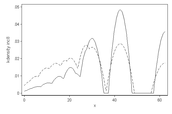
Kernel-density of inc8 with inverse propensity weighting. (Note shown in text.)
twoway kdensity inc8 if catholic==1 [aw=pscorewgt] || ///
	kdensity inc8 if catholic==0 [aw=pscorewgt], ///
	legend(off) scheme(lean1)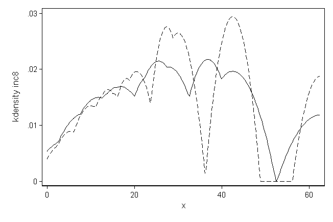
Figure 13.3, Part A on page 327.
twoway kdensity math8 if catholic==1 || ///
	kdensity math8 if catholic==0, ///
	legend(off) scheme(lean1)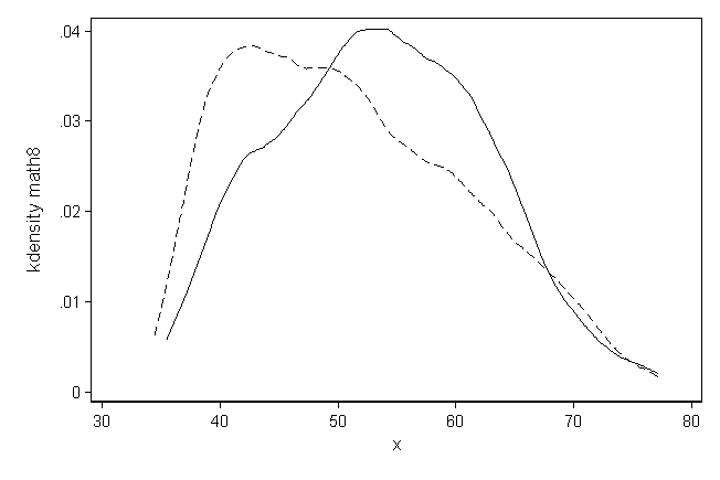
Figure 13.3, Part B on page 327.
twoway kdensity math8 if catholic==1 [aw=pscorewgt] || ///
	kdensity math8 if catholic==0 [aw=pscorewgt], ///
	legend(off) scheme(lean1)