use https://stats.idre.ucla.edu/stat/stata/examples/methods_matter/chapter7/sfa
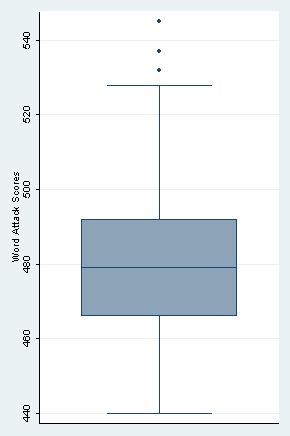
Descriptive statistics for the variable wattack. Notice the floor effect which cannot be resolved by a straightforward transformation. (Note these analyses are not shown in the text.)
sum wattack, detail

                    word attack posttest
-------------------------------------------------------------
      Percentiles      Smallest
 1%          440            440
 5%          440            440
10%          449            440       Obs                2334
25%          466            440       Sum of Wgt.        2334

50%          479                      Mean           478.5193
                        Largest       Std. Dev.      19.87872
75%          492            537
90%          503            537       Variance       395.1636
95%          509            545       Skewness       -.165475
99%          525            545       Kurtosis       2.801111


graph box wattack, medtype(line) ytitle(Word Attack Scores) ysize(3) xsize(2)
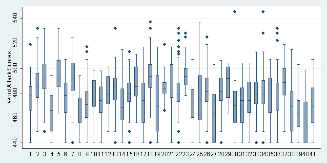
Descriptive analyses of wattack by school (schid). Note the floor effect is present in most schools. (Not shown in text.)
table schid, contents(mean wattack sd wattack min wattack max wattack freq)

--------------------------------------------------------------------------------
school id | mean(watt~k)   sd(wattack)  min(wattack)  max(wattack)         Freq.
----------+---------------------------------------------------------------------
        1 |      475.731      16.15988           440           519            52
        2 |      486.603      15.31063           449           532           116
        3 |      491.368       16.8469           449           532            68
        4 |      462.912      16.55179           440           494            34
        5 |      495.085      14.96783           464           532            47
        6 |      475.115      18.07763           440           507            87
        7 |       491.53      16.19119           440           525            83
        8 |        467.5       13.9412           440           494            22
        9 |      471.105       17.6963           440           517            95
       10 |      474.556      19.07744           440           498            27
       11 |      472.186      16.68797           440           498            43
       12 |      478.963      13.21852           449           501            27
       13 |      483.871      14.56414           440           532            62
       14 |      469.889      17.18767           440           515            36
       15 |      479.556      15.97128           440           513            54
       16 |       486.75      14.86967           456           511            36
       17 |      472.951      22.71998           440           517            41
       18 |      492.596      17.52095           440           537           109
       19 |      468.739      23.85604           440           517            23
       20 |       484.75      11.13494           466           519            20
       21 |      487.231      19.07008           440           517           134
       22 |      480.274      18.01826           440           532           106
       23 |      495.333      12.11611           478           528            36
       24 |      470.771      17.15045           440           507            48
       25 |      476.019      23.51344           440           537            52
       26 |       480.97      18.02645           440           525            66
       27 |      462.951      19.46015           440           503            41
       28 |      480.839      15.78236           440           506            56
       29 |        488.1      15.19832           464           504            10
       30 |      469.625      22.41857           440           545            24
       31 |      471.525      17.96627           440           504            61
       32 |      474.724      17.77224           440           504            58
       33 |      478.878      19.19921           440           513            41
       34 |      479.418      19.18507           440           545            79
       35 |      474.421      18.73494           440           507            57
       36 |      476.929      20.63214           440           532            85
       37 |       487.19      16.92756           449           519            58
       38 |      468.189      21.31749           440           515            37
       39 |      464.361      16.32553           440           503            36
       40 |      459.252      16.97395           440           498           107
       41 |      468.933      17.35362           440           507            60
--------------------------------------------------------------------------------


graph box wattack, medtype(line) over(schid) ytitle(Word Attack Scores) ysize(2) xsize(4)
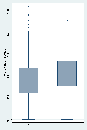
Descriptive analyses of wattack by experimental condition (sfa). (Not shown in text.)
bysort sfa: sum wattack, detail

------------------------------------------------------------------------------------------
-> sfa = 0

                    word attack posttest
-------------------------------------------------------------
      Percentiles      Smallest
 1%          440            440
 5%          440            440
10%          440            440       Obs                1118
25%          464            440       Sum of Wgt.        1118

50%          476                      Mean           474.8247
                        Largest       Std. Dev.      20.05239
75%          488            532
90%          500            537       Variance       402.0982
95%          506            545       Skewness      -.0207681
99%          525            545       Kurtosis       2.808253

------------------------------------------------------------------------------------------
-> sfa = 1

                    word attack posttest
-------------------------------------------------------------
      Percentiles      Smallest
 1%          440            440
 5%          440            440
10%          456            440       Obs                1216
25%          471            440       Sum of Wgt.        1216

50%          482                      Mean           481.9161
                        Largest       Std. Dev.      19.10511
75%          494            532
90%          506            532       Variance       365.0053
95%          511            532       Skewness       -.280702
99%          522            537       Kurtosis       2.936778


graph box wattack, medtype(line) over(sfa) ytitle(Word Attack Scores) ysize(3) xsize(2)
Model #1 from Table 7.1 on page 114.
xtreg wattack, i(schid)

Random-effects GLS regression                   Number of obs      =      2334
Group variable: schid                           Number of groups   =        41

R-sq:  within  = 0.0000                         Obs per group: min =        10
       between = 0.0000                                        avg =      56.9
       overall = 0.0000                                        max =       134

Random effects u_i ~ Gaussian                   Wald chi2(0)       =         .
corr(u_i, X)       = 0 (assumed)                Prob > chi2        =         .

------------------------------------------------------------------------------
     wattack |      Coef.   Std. Err.      z    P>|z|     [95% Conf. Interval]
-------------+----------------------------------------------------------------
       _cons |   477.5356   1.447118   329.99   0.000     474.6994    480.3719
-------------+----------------------------------------------------------------
     sigma_u |  8.8705267
     sigma_e |  17.725757
         rho |  .20027618   (fraction of variance due to u_i)
------------------------------------------------------------------------------

* variance of sigma u
display e(sigma_u)^2
78.686244

* variance of sigma e
display e(sigma_e)^2
314.20244
Model #2 from Table 7.1 on page 114.
xtreg wattack sfa, i(schid)

Random-effects GLS regression                   Number of obs      =      2334
Group variable: schid                           Number of groups   =        41

R-sq:  within  = 0.0000                         Obs per group: min =        10
       between = 0.0486                                        avg =      56.9
       overall = 0.0318                                        max =       134

Random effects u_i ~ Gaussian                   Wald chi2(1)       =      2.33
corr(u_i, X)       = 0 (assumed)                Prob > chi2        =    0.1271

------------------------------------------------------------------------------
     wattack |      Coef.   Std. Err.      z    P>|z|     [95% Conf. Interval]
-------------+----------------------------------------------------------------
         sfa |   4.362971   2.859467     1.53   0.127    -1.241483    9.967424
       _cons |   475.3036   2.045759   232.34   0.000      471.294    479.3132
-------------+----------------------------------------------------------------
     sigma_u |  8.7525004
     sigma_e |  17.725757
         rho |  .19601985   (fraction of variance due to u_i)
------------------------------------------------------------------------------

* variance sigma u
display e(sigma_u)^2
76.606263

* variance sigma e
display e(sigma_e)^2
314.20244
Model #3 from Table 7.1 on page 114. The variable sch_ppvt is the within-school average of ppvt based on the full sample, rather than the subsample analyzed here, see footnote 15 on page 127.
xtreg wattack sfa sch_ppvt, i(schid)

Random-effects GLS regression                   Number of obs      =      2334
Group variable: schid                           Number of groups   =        41

R-sq:  within  = 0.0000                         Obs per group: min =        10
       between = 0.3820                                        avg =      56.9
       overall = 0.0914                                        max =       134

Random effects u_i ~ Gaussian                   Wald chi2(2)       =     23.58
corr(u_i, X)       = 0 (assumed)                Prob > chi2        =    0.0000

------------------------------------------------------------------------------
     wattack |      Coef.   Std. Err.      z    P>|z|     [95% Conf. Interval]
-------------+----------------------------------------------------------------
         sfa |   3.572224    2.33971     1.53   0.127    -1.013523     8.15797
    sch_ppvt |   .6228176    .139824     4.45   0.000     .3487675    .8968676
       _cons |   419.8154   12.55807    33.43   0.000      395.202    444.4287
-------------+----------------------------------------------------------------
     sigma_u |  6.9693079
     sigma_e |  17.725757
         rho |  .13388857   (fraction of variance due to u_i)
------------------------------------------------------------------------------

* variance sigma u
display e(sigma_u)^2
48.571253

* variance sigma e
display e(sigma_e)^2
314.20244
Model #3 using the within-school averages of prior ppvt score (new variable schavgppvt) from the analytic subsample instead of sch_ppvt. (Not shown in text, this analysis is mentioned in footnote 15 on page 127.)
bysort schid: egen schavgppvt = mean(ppvt)

xtreg wattack sfa schavgppvt, i(schid)

Random-effects GLS regression                   Number of obs      =      2334
Group variable: schid                           Number of groups   =        41

R-sq:  within  = 0.0000                         Obs per group: min =        10
       between = 0.4003                                        avg =      56.9
       overall = 0.0977                                        max =       134

Random effects u_i ~ Gaussian                   Wald chi2(2)       =     25.57
corr(u_i, X)       = 0 (assumed)                Prob > chi2        =    0.0000

------------------------------------------------------------------------------
     wattack |      Coef.   Std. Err.      z    P>|z|     [95% Conf. Interval]
-------------+----------------------------------------------------------------
         sfa |   3.218344   2.311869     1.39   0.164    -1.312837    7.749524
  schavgppvt |   .6023257   .1293094     4.66   0.000      .348884    .8557674
       _cons |   421.6086    11.6332    36.24   0.000     398.8079    444.4092
-------------+----------------------------------------------------------------
     sigma_u |  6.8490081
     sigma_e |  17.725757
         rho |  .12990151   (fraction of variance due to u_i)
------------------------------------------------------------------------------
The following models show various ways of controlling for individual- and school-level ppvt. None of the models shown below are displayed in the text.
Controlling for individual-level ppvt, deviated from the grand mean (new variable ppvt_devgm).
sum ppvt

    Variable |       Obs        Mean    Std. Dev.       Min        Max
-------------+--------------------------------------------------------
        ppvt |      2334     90.4006    15.00082         40        144


gen ppvt_devgm = ppvt-90.4006
xtreg wattack sfa ppvt_devgm, i(schid)

Random-effects GLS regression                   Number of obs      =      2334
Group variable: schid                           Number of groups   =        41

R-sq:  within  = 0.1101                         Obs per group: min =        10
       between = 0.3960                                        avg =      56.9
       overall = 0.1820                                        max =       134

Random effects u_i ~ Gaussian                   Wald chi2(2)       =    308.21
corr(u_i, X)       = 0 (assumed)                Prob > chi2        =    0.0000

------------------------------------------------------------------------------
     wattack |      Coef.   Std. Err.      z    P>|z|     [95% Conf. Interval]
-------------+----------------------------------------------------------------
         sfa |   3.440921   2.297268     1.50   0.134    -1.061642    7.943485
  ppvt_devgm |   .4851754   .0278075    17.45   0.000     .4306737    .5396771
       _cons |   475.9076   1.642957   289.67   0.000     472.6875    479.1278
-------------+----------------------------------------------------------------
     sigma_u |  6.9082397
     sigma_e |  16.725172
         rho |  .14574142   (fraction of variance due to u_i)
------------------------------------------------------------------------------
Controlling for individual-level ppvt by including deviations of individual scores from school-average scores (new variable ppvt_devsm) and school-average scores from the grand mean (new variable schavgppvt_devgm).
gen ppvt_devsm = ppvt-schavgppvt
gen schavgppvt_devgm = schavgppvt-90.4006

xtreg wattack sfa ppvt_devsm schavgppvt_devgm, i(schid)

Random-effects GLS regression                   Number of obs      =      2334
Group variable: schid                           Number of groups   =        41

R-sq:  within  = 0.1101                         Obs per group: min =        10
       between = 0.4004                                        avg =      56.9
       overall = 0.1835                                        max =       134

Random effects u_i ~ Gaussian                   Wald chi2(3)       =    308.73
corr(u_i, X)       = 0 (assumed)                Prob > chi2        =    0.0000

------------------------------------------------------------------------------
     wattack |      Coef.   Std. Err.      z    P>|z|     [95% Conf. Interval]
-------------+----------------------------------------------------------------
         sfa |   3.187396   2.331659     1.37   0.172    -1.382572    7.757363
  ppvt_devsm |   .4794657   .0284703    16.84   0.000     .4236648    .5352666
schavgppvt~m |   .6030759   .1303864     4.63   0.000     .3475233    .8586285
       _cons |   476.0634   1.664848   285.95   0.000     472.8003    479.3264
-------------+----------------------------------------------------------------
     sigma_u |  6.9726021
     sigma_e |  16.725172
         rho |  .14806577   (fraction of variance due to u_i)
------------------------------------------------------------------------------
Controlling for school-average ppvt deviated from the grand mean (schavgppvt_devgm).
xtreg wattack sfa schavgppvt_devgm, i(schid)

Random-effects GLS regression                   Number of obs      =      2334
Group variable: schid                           Number of groups   =        41

R-sq:  within  = 0.0000                         Obs per group: min =        10
       between = 0.4003                                        avg =      56.9
       overall = 0.0977                                        max =       134

Random effects u_i ~ Gaussian                   Wald chi2(2)       =     25.57
corr(u_i, X)       = 0 (assumed)                Prob > chi2        =    0.0000

------------------------------------------------------------------------------
     wattack |      Coef.   Std. Err.      z    P>|z|     [95% Conf. Interval]
-------------+----------------------------------------------------------------
         sfa |   3.218344   2.311869     1.39   0.164    -1.312837    7.749524
schavgppvt~m |   .6023257   .1293094     4.66   0.000      .348884    .8557674
       _cons |   476.0592   1.650323   288.46   0.000     472.8246    479.2937
-------------+----------------------------------------------------------------
     sigma_u |  6.8490081
     sigma_e |  17.725757
         rho |  .12990151   (fraction of variance due to u_i)
------------------------------------------------------------------------------