Version info: Code for this page was tested in Stata 12.1.
For this chapter, you will need to use the syntax provided in Appendix A to access the School and Mice datasets.
Figure 18.2, page 466
* Figure 18.2, page 466
sort SCHOOL
by SCHOOL: egen ordervar = median(MATH)
egen id = group(ordervar SCHOOL)
graph box MATH, over(id)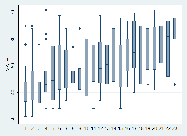
Table 18.2, page 468 Estimated coefficients from three naive linear regression models ignoring the hierarchical structure of the school data. Note that for Model 3, we believe there is a typo where the coefficient for “Three hours” was copied for “Four or more hours”.
* Table 18.2, page 468
regress MATH i.iSCHTYPE
regress MATH i.iSCHTYPE SES
regress MATH i.iSCHTYPE SES i.iHOMEW

. regress MATH i.iSCHTYPE

      Source |       SS       df       MS              Number of obs =     519
-------------+------------------------------           F(  1,   517) =   74.89
       Model |  7517.11179     1  7517.11179           Prob > F      =  0.0000
    Residual |  51890.9345   517  100.369312           R-squared     =  0.1265
-------------+------------------------------           Adj R-squared =  0.1248
       Total |  59408.0462   518  114.687348           Root MSE      =  10.018

------------------------------------------------------------------------------
        MATH |      Coef.   Std. Err.      t    P>|t|     [95% Conf. Interval]
-------------+----------------------------------------------------------------
  1.iSCHTYPE |  -7.805556   .9019425    -8.65   0.000    -9.577479   -6.033634
       _cons |    56.4901   .7048956    80.14   0.000     55.10529    57.87491
------------------------------------------------------------------------------

. regress MATH i.iSCHTYPE SES

      Source |       SS       df       MS              Number of obs =     519
-------------+------------------------------           F(  2,   516) =   86.56
       Model |  14923.9649     2  7461.98243           Prob > F      =  0.0000
    Residual |  44484.0814   516    86.20946           R-squared     =  0.2512
-------------+------------------------------           Adj R-squared =  0.2483
       Total |  59408.0462   518  114.687348           Root MSE      =  9.2849

------------------------------------------------------------------------------
        MATH |      Coef.   Std. Err.      t    P>|t|     [95% Conf. Interval]
-------------+----------------------------------------------------------------
  1.iSCHTYPE |  -2.690174   1.001647    -2.69   0.007    -4.657982   -.7223663
         SES |   5.144264   .5549883     9.27   0.000      4.05395    6.234579
       _cons |   53.37222   .7347965    72.64   0.000     51.92866    54.81578
------------------------------------------------------------------------------

. regress MATH i.iSCHTYPE SES i.iHOMEW

      Source |       SS       df       MS              Number of obs =     519
-------------+------------------------------           F(  7,   511) =   39.29
       Model |   20787.198     7  2969.59972           Prob > F      =  0.0000
    Residual |  38620.8482   511  75.5789593           R-squared     =  0.3499
-------------+------------------------------           Adj R-squared =  0.3410
       Total |  59408.0462   518  114.687348           Root MSE      =  8.6936

------------------------------------------------------------------------------
        MATH |      Coef.   Std. Err.      t    P>|t|     [95% Conf. Interval]
-------------+----------------------------------------------------------------
  1.iSCHTYPE |  -1.604598   .9512725    -1.69   0.092    -3.473485    .2642879
         SES |    4.27564   .5316148     8.04   0.000      3.23122    5.320059
             |
      iHOMEW |
          1  |  -1.390219   1.463883    -0.95   0.343    -4.266189    1.485751
          2  |   .2264091   1.578583     0.14   0.886    -2.874903    3.327721
          3  |   5.208512   1.852822     2.81   0.005     1.568426    8.848598
          4  |   7.560103   1.889684     4.00   0.000     3.847598    11.27261
          5  |   8.073905     1.9118     4.22   0.000     4.317949    11.82986
             |
       _cons |   51.37485   1.508053    34.07   0.000     48.41211     54.3376
------------------------------------------------------------------------------
Table 18.3, page 472 Estimated coefficients from three random slope regression models accounting for the hierarchical structure of the school data.
* Table 18.3, page 472
xtmixed MATH i.iSCHTYPE || SCHOOL:
xtmixed MATH i.iSCHTYPE SES || SCHOOL:
xtmixed MATH i.iSCHTYPE SES i.iHOMEW || SCHOOL:

. xtmixed MATH i.iSCHTYPE || SCHOOL:

Performing EM optimization:

Performing gradient-based optimization:

Iteration 0:   log likelihood =  -1896.834
Iteration 1:   log likelihood =  -1896.834

Computing standard errors:

Mixed-effects ML regression                     Number of obs      =       519
Group variable: SCHOOL                          Number of groups   =        23

                                                Obs per group: min =         5
                                                               avg =      22.6
                                                               max =        67


                                                Wald chi2(1)       =      8.37
Log likelihood =  -1896.834                     Prob > chi2        =    0.0038

------------------------------------------------------------------------------
        MATH |      Coef.   Std. Err.      z    P>|z|     [95% Conf. Interval]
-------------+----------------------------------------------------------------
  1.iSCHTYPE |  -5.917381   2.045617    -2.89   0.004    -9.926718   -1.908045
       _cons |   54.67714   1.666538    32.81   0.000     51.41078    57.94349
------------------------------------------------------------------------------

------------------------------------------------------------------------------
  Random-effects Parameters  |   Estimate   Std. Err.     [95% Conf. Interval]
-----------------------------+------------------------------------------------
SCHOOL: Identity             |
                   sd(_cons) |    4.14692   .7461234      2.914577    5.900324
-----------------------------+------------------------------------------------
                sd(Residual) |   9.012207   .2858282      8.469051    9.590198
------------------------------------------------------------------------------
LR test vs. linear regression: chibar2(01) =    69.18 Prob >= chibar2 = 0.0000

. xtmixed MATH i.iSCHTYPE SES || SCHOOL:

Performing EM optimization:

Performing gradient-based optimization:

Iteration 0:   log likelihood = -1873.2488
Iteration 1:   log likelihood = -1873.2488

Computing standard errors:

Mixed-effects ML regression                     Number of obs      =       519
Group variable: SCHOOL                          Number of groups   =        23

                                                Obs per group: min =         5
                                                               avg =      22.6
                                                               max =        67


                                                Wald chi2(2)       =     63.07
Log likelihood = -1873.2488                     Prob > chi2        =    0.0000

------------------------------------------------------------------------------
        MATH |      Coef.   Std. Err.      z    P>|z|     [95% Conf. Interval]
-------------+----------------------------------------------------------------
  1.iSCHTYPE |  -2.439539   1.765271    -1.38   0.167    -5.899407     1.02033
         SES |   4.157041   .5842519     7.12   0.000     3.011928    5.302153
       _cons |   52.80351   1.407527    37.52   0.000     50.04481    55.56221
------------------------------------------------------------------------------

------------------------------------------------------------------------------
  Random-effects Parameters  |   Estimate   Std. Err.     [95% Conf. Interval]
-----------------------------+------------------------------------------------
SCHOOL: Identity             |
                   sd(_cons) |   3.286817   .6568919      2.221556    4.862882
-----------------------------+------------------------------------------------
                sd(Residual) |   8.668816   .2751664      8.145934    9.225262
------------------------------------------------------------------------------
LR test vs. linear regression: chibar2(01) =    36.42 Prob >= chibar2 = 0.0000

. xtmixed MATH i.iSCHTYPE SES i.iHOMEW || SCHOOL:

Performing EM optimization:

Performing gradient-based optimization:

Iteration 0:   log likelihood = -1836.8366
Iteration 1:   log likelihood = -1836.8366

Computing standard errors:

Mixed-effects ML regression                     Number of obs      =       519
Group variable: SCHOOL                          Number of groups   =        23

                                                Obs per group: min =         5
                                                               avg =      22.6
                                                               max =        67


                                                Wald chi2(7)       =    148.88
Log likelihood = -1836.8366                     Prob > chi2        =    0.0000

------------------------------------------------------------------------------
        MATH |      Coef.   Std. Err.      z    P>|z|     [95% Conf. Interval]
-------------+----------------------------------------------------------------
  1.iSCHTYPE |  -1.634042    1.71019    -0.96   0.339    -4.985953    1.717868
         SES |    3.48564   .5527899     6.31   0.000     2.402191    4.569088
             |
      iHOMEW |
          1  |  -1.296386   1.414758    -0.92   0.359     -4.06926    1.476489
          2  |   .7045507   1.530507     0.46   0.645    -2.295187    3.704289
          3  |   5.297748   1.787483     2.96   0.003     1.794345    8.801151
          4  |   7.632283   1.820814     4.19   0.000     4.063553    11.20101
          5  |   7.713808   1.855085     4.16   0.000     4.077909    11.34971
             |
       _cons |   50.98939    1.85495    27.49   0.000     47.35376    54.62503
------------------------------------------------------------------------------

------------------------------------------------------------------------------
  Random-effects Parameters  |   Estimate   Std. Err.     [95% Conf. Interval]
-----------------------------+------------------------------------------------
SCHOOL: Identity             |
                   sd(_cons) |   3.230354   .6381913       2.19324    4.757887
-----------------------------+------------------------------------------------
                sd(Residual) |   8.066908   .2562394      7.580002    8.585091
------------------------------------------------------------------------------
LR test vs. linear regression: chibar2(01) =    35.89 Prob >= chibar2 = 0.0000
Figure 18.3 is not reproduced.
Table 18.4, page 480 is not reproduced — it is just the AICs from running all possible sets of 2 and 3 predictors in xtmixed.
Figure 18.4, page 483 Weight over time for 14 Mice.
* Figure 18.4, page 483
twoway line WEIGHT DAY, lstyle(ID)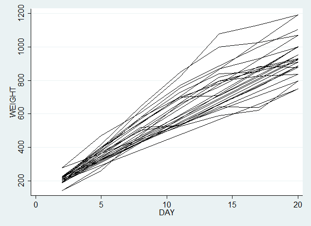
Table 18.5, page 485 Estimates for random intercept and random slope models with different correlation structures. Note that these are complex random effects models to be fitting on only 14 mice. The parameter estimates vary between packages, with some reporting Errors or warnings in the optimization.
* Table 18.5, page 485
xtmixed WEIGHT DAY || ID: DAY, mle residuals(ar 1, t(DAY)) nolrtest nolog nogroup
* log likelihood, AIC, BIC (note nondefault N)
estat ic, n(14)

xtmixed WEIGHT DAY || ID: DAY, mle residuals(exchangeable, t(DAY)) nolrtest nogroup
estat ic, n(14)

. xtmixed WEIGHT DAY || ID: DAY, mle residuals(ar 1, t(DAY)) nolrtest nolog nogroup
Note: time gaps exist in the estimation data

Mixed-effects ML regression                     Number of obs      =        98
                                                Wald chi2(1)       =    412.99
Log likelihood = -541.87375                     Prob > chi2        =    0.0000

------------------------------------------------------------------------------
      WEIGHT |      Coef.   Std. Err.      z    P>|z|     [95% Conf. Interval]
-------------+----------------------------------------------------------------
         DAY |   41.05531    2.02023    20.32   0.000     37.09573    45.01488
       _cons |   156.8233   22.00866     7.13   0.000     113.6871    199.9595
------------------------------------------------------------------------------

------------------------------------------------------------------------------
  Random-effects Parameters  |   Estimate   Std. Err.     [95% Conf. Interval]
-----------------------------+------------------------------------------------
ID: Independent              |
                     sd(DAY) |   5.071184   1.621431      2.709887     9.49003
                   sd(_cons) |   5.02e-07          .             .           .
-----------------------------+------------------------------------------------
Residual: AR(1)              |
                         rho |   .8948443   .0371771      .7932106    .9479758
                       sd(e) |   77.01422   12.31915      56.28766    105.3728
------------------------------------------------------------------------------

. * log likelihood, AIC, BIC (note nondefault N)
. estat ic, n(14)

-----------------------------------------------------------------------------
       Model |    Obs    ll(null)   ll(model)     df          AIC         BIC
-------------+---------------------------------------------------------------
           . |     14           .   -541.8737      5     1093.747    1096.943
-----------------------------------------------------------------------------
               Note:  N=14 used in calculating BIC

.
. xtmixed WEIGHT DAY || ID: DAY, mle residuals(exchangeable, t(DAY)) nolrtest nogroup
Note: t() not required for this residual structure; ignored

Obtaining starting values by EM:

Performing gradient-based optimization:

Iteration 0:   log likelihood = -559.76833
Iteration 1:   log likelihood =   -559.262
Iteration 2:   log likelihood = -559.21086
Iteration 3:   log likelihood = -559.20315
Iteration 4:   log likelihood = -559.20143  (backed up)
Iteration 5:   log likelihood = -559.20059  (backed up)
Iteration 6:   log likelihood = -559.20038  (backed up)
Iteration 7:   log likelihood = -559.20028  (backed up)
Iteration 8:   log likelihood = -559.20025  (backed up)
numerical derivatives are approximate
nearby values are missing
Iteration 9:   log likelihood = -559.20024  (not concave)
numerical derivatives are approximate
nearby values are missing
Iteration 10:  log likelihood = -559.20023  (not concave)
numerical derivatives are approximate
nearby values are missing
Iteration 11:  log likelihood = -559.20022  (not concave)
numerical derivatives are approximate
nearby values are missing
Iteration 12:  log likelihood = -559.19951
numerical derivatives are approximate
nearby values are missing
Iteration 13:  log likelihood = -559.15415  (not concave)
numerical derivatives are approximate
nearby values are missing
Iteration 14:  log likelihood = -559.15414  (backed up)
numerical derivatives are approximate
nearby values are missing
Iteration 15:  log likelihood = -559.15315
numerical derivatives are approximate
nearby values are missing
Iteration 16:  log likelihood = -559.15315  (not concave)
numerical derivatives are approximate
nearby values are missing
Iteration 17:  log likelihood = -559.15315  (backed up)

Computing standard errors:

Mixed-effects ML regression                     Number of obs      =        98
                                                Wald chi2(1)       =    361.72
Log likelihood = -559.15315                     Prob > chi2        =    0.0000

------------------------------------------------------------------------------
      WEIGHT |      Coef.   Std. Err.      z    P>|z|     [95% Conf. Interval]
-------------+----------------------------------------------------------------
         DAY |   41.05442   2.158596    19.02   0.000     36.82365    45.28519
       _cons |   180.4116   11.31704    15.94   0.000     158.2306    202.5926
------------------------------------------------------------------------------

------------------------------------------------------------------------------
  Random-effects Parameters  |   Estimate   Std. Err.     [95% Conf. Interval]
-----------------------------+------------------------------------------------
ID: Independent              |
                     sd(DAY) |   7.100342   1.341837      4.902499     10.2835
                   sd(_cons) |   .0004224          .             .           .
-----------------------------+------------------------------------------------
Residual: Exchangeable       |
                       sd(e) |   56.57587   4.364924       48.6362    65.81166
                     corr(e) |  -.1666667    .000035     -.1667352   -.1665981
------------------------------------------------------------------------------

. estat ic, n(14)

-----------------------------------------------------------------------------
       Model |    Obs    ll(null)   ll(model)     df          AIC         BIC
-------------+---------------------------------------------------------------
           . |     14           .   -559.1531      5     1128.306    1131.502
-----------------------------------------------------------------------------
               Note:  N=14 used in calculating BIC