Figure 5.1, page 146.
NOTE: The graph does not match up exactly.
use https://stats.idre.ucla.edu/stat/stata/examples/rwg/crfe, clear
graph twoway (scatter crfe depth) (mband crfe depth, band(5)), ///
	xlabel(0(5)25) ylabel(0(2)10) xline(5 10 15 20)
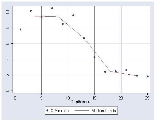
Table 5.1, page 147. The command egen is used to create the new variables because unlike gen, egen can use functions, such as median, to create variables.
use https://stats.idre.ucla.edu/stat/stata/examples/rwg/crfe, clear

gen band=_n
recode band 1/2=1 3/5=2 6/7=3 8/10=4 11/13=5
(12 changes made)

egen mddepth=median(depth), by(band)
egen mdcrfe=median(crfe), by(band)
list depth crfe mddepth mdcrfe

        depth       crfe    mddepth     mdcrfe
  1.        1        7.8          2          9
  2.        3       10.2          2          9
  3.        9        8.5          7        9.4
  4.        5        9.4          7        9.4
  5.        7       10.5          7        9.4
  6.       13        6.7         12       8.15
  7.       11        9.6         12       8.15
  8.       17        2.4         17        2.5
  9.       19        2.5         17        2.5
 10.       15        4.3         17        2.5
 11.       25        1.8         23        1.9
 12.       23        1.9         23        1.9
 13.       21        2.6         23        1.9
Table 5.2, page 155.
Note: In Stata, ln(x)=log(x), in other words, log(x) defaults to natural log instead of log base 10. If you want log base 10, use log10(x).
use https://stats.idre.ucla.edu/stat/stata/examples/rwg/concord1, clear

gen wtr81_3=(water81)^.3
label variable wtr81_3 "water81 to the .3 power"
gen wtr80_3=(water80)^.3
label variable wtr80_3 "water80 to the .3 power"
gen inc_3=(income)^.3
label variable inc_3 "income to the .3 power"
gen logpeop=log(peop81)
label variable logpeop "log of peop81"
gen clogpeop=log(peop81/peop80)
label variable clogpeop "log of peop81/peop80"
regress wtr81_3 inc_3 wtr80_3 educat retire logpeop clogpeop

  Source |       SS       df       MS                  Number of obs =     496
---------+------------------------------               F(  6,   489) =  209.51
   Model |   1310.1171     6   218.35285               Prob > F      =  0.0000
Residual |  509.636644   489  1.04220173               R-squared     =  0.7199
---------+------------------------------               Adj R-squared =  0.7165
   Total |  1819.75374   495  3.67627019               Root MSE      =  1.0209

------------------------------------------------------------------------------
 wtr81_3 |      Coef.   Std. Err.       t     P>|t|       [95% Conf. Interval]
---------+--------------------------------------------------------------------
   inc_3 |     .51572   .1297219      3.976   0.000        .260839    .7706011
 wtr80_3 |   .6255023   .0290827     21.508   0.000       .5683599    .6826446
  educat |  -.0361339   .0160111     -2.257   0.024       -.067593   -.0046749
  retire |   .1013897   .1189905      0.852   0.395       -.132406    .3351855
 logpeop |   .7146849   .1104854      6.469   0.000       .4976001    .9317696
clogpeop |   .9156945   .2627408      3.485   0.001       .3994542    1.431935
   _cons |   1.856262   .3849294      4.822   0.000       1.099942    2.612581
------------------------------------------------------------------------------
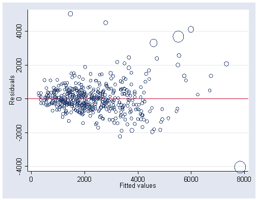
Figure 5.7, page 156.
NOTE: You cannot use the avplot with the [w=d] option, which is why the graph command was used. If you wanted to produce this plot without the scaling (which is the [w=d] option), you could use avplot.
use https://stats.idre.ucla.edu/stat/stata/examples/rwg/concord1, clear

quietly regress water81 income water80 educat retire peop81 cpeop peop80
predict yhat
predict e, residual
predict d, cooksd
gen cook = .
replace cook = (99/4)*d*(d+1)^2 + 1 if d <=1
replace cook = 100 if d >1
graph twoway (scatter e yhat [w=cook], msymbol(oh)), ylabel(-4000(2000)4000) yline(0)
use https://stats.idre.ucla.edu/stat/stata/examples/rwg/concord1, clear

gen wtr81_3=(water81)^.3
gen wtr80_3=(water80)^.3
gen inc_3=(income)^.3
gen logpeop=log(peop81)
gen clogpeop=log(peop81/peop80)
regress wtr81_3 inc_3 wtr80_3 educat retire logpeop clogpeop

  Source |       SS       df       MS                  Number of obs =     496
---------+------------------------------               F(  6,   489) =  209.51
   Model |   1310.1171     6   218.35285               Prob > F      =  0.0000
Residual |  509.636644   489  1.04220173               R-squared     =  0.7199
---------+------------------------------               Adj R-squared =  0.7165
   Total |  1819.75374   495  3.67627019               Root MSE      =  1.0209

------------------------------------------------------------------------------
 wtr81_3 |      Coef.   Std. Err.       t     P>|t|       [95% Conf. Interval]
---------+--------------------------------------------------------------------
   inc_3 |     .51572   .1297219      3.976   0.000        .260839    .7706011
 wtr80_3 |   .6255023   .0290827     21.508   0.000       .5683599    .6826446
  educat |  -.0361339   .0160111     -2.257   0.024       -.067593   -.0046749
  retire |   .1013897   .1189905      0.852   0.395       -.132406    .3351855
 logpeop |   .7146849   .1104854      6.469   0.000       .4976001    .9317696
clogpeop |   .9156945   .2627408      3.485   0.001       .3994542    1.431935
   _cons |   1.856262   .3849294      4.822   0.000       1.099942    2.612581
------------------------------------------------------------------------------

predict yhat
predict e, residual
predict d, cooksd
gen cook = .
replace cook = (99/4)*d*(d+1)^2 + 1 if d <=1
replace cook = 100 if d >1
graph twoway (scatter e yhat [w=cook], msymbol(oh)), ylabel(-4(2)4) xlabel(6(2)14) yline(0)
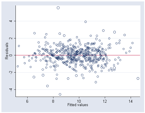
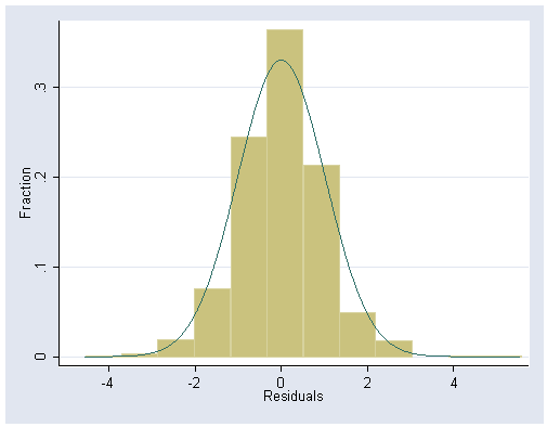
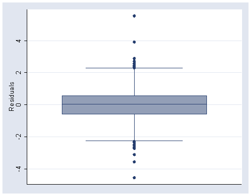
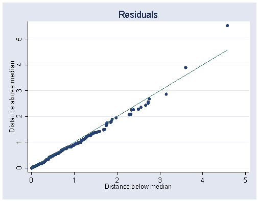
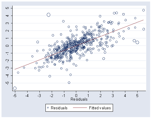
Figure 5.8, page 157.
use https://stats.idre.ucla.edu/stat/stata/examples/rwg/concord1, clear

gen wtr81_3=(water81)^.3
gen wtr80_3=(water80)^.3
gen inc_3=(income)^.3
gen logpeop=log(peop81)
gen clogpeop=log(peop81/peop80)
regress wtr81_3 inc_3 wtr80_3 educat retire logpeop clogpeop

  Source |       SS       df       MS                  Number of obs =     496
---------+------------------------------               F(  6,   489) =  209.51
   Model |   1310.1171     6   218.35285               Prob > F      =  0.0000
Residual |  509.636644   489  1.04220173               R-squared     =  0.7199
---------+------------------------------               Adj R-squared =  0.7165
   Total |  1819.75374   495  3.67627019               Root MSE      =  1.0209

------------------------------------------------------------------------------
 wtr81_3 |      Coef.   Std. Err.       t     P>|t|       [95% Conf. Interval]
---------+--------------------------------------------------------------------
   inc_3 |     .51572   .1297219      3.976   0.000        .260839    .7706011
 wtr80_3 |   .6255023   .0290827     21.508   0.000       .5683599    .6826446
  educat |  -.0361339   .0160111     -2.257   0.024       -.067593   -.0046749
  retire |   .1013897   .1189905      0.852   0.395       -.132406    .3351855
 logpeop |   .7146849   .1104854      6.469   0.000       .4976001    .9317696
clogpeop |   .9156945   .2627408      3.485   0.001       .3994542    1.431935
   _cons |   1.856262   .3849294      4.822   0.000       1.099942    2.612581
------------------------------------------------------------------------------

predict e, residual
graph e, norm xlabel(-4 (-2) 4) ylabel(0 (.1) .3) bin(12)
Histogram:
histogram e, norm xlabel(-4(2)4) ylabel(0(.1).3) bin(12) fraction
Boxplot:
graph box e, ylabel(-4(2)4)
Symplot:
symplot e, xlabel(0(1)5) ylabel(0(1)5)
Quantile-normal plot:
qnorm e, ylabel(-4(2)4) xlabel(-2 0 2)
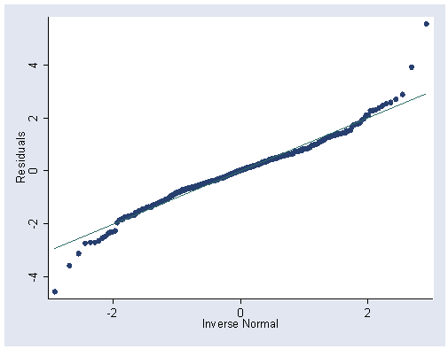
Figure 5.9, page 157.
Note: yresid, xresid, d and y-hat need to be dropped or else Stata will complain that they have already been defined. You can also use the use https://stats.idre.ucla.edu/stat/stata/examples/rwg/concord1, clear command and re-enter wtr81_3 wtr80_3 and inc_3 instead of dropping yresid, xresid, d and yhat. A third option would be to save the preceding data set with a new name and then to open concord1, saving it with a new name. The clear option was used above (when starting the histogram).
regress wtr81_3 wtr80_3 retire educat logpeop clogpeop

  Source |       SS       df       MS                  Number of obs =     496
---------+------------------------------               F(  5,   490) =  240.97
   Model |  1293.64483     5  258.728966               Prob > F      =  0.0000
Residual |  526.108911   490  1.07369166               R-squared     =  0.7109
---------+------------------------------               Adj R-squared =  0.7079
   Total |  1819.75374   495  3.67627019               Root MSE      =  1.0362

------------------------------------------------------------------------------
 wtr81_3 |      Coef.   Std. Err.       t     P>|t|       [95% Conf. Interval]
---------+--------------------------------------------------------------------
 wtr80_3 |   .6475596   .0289766     22.348   0.000       .5906259    .7044933
  retire |  -.0368787   .1155006     -0.319   0.750      -.2638162    .1900588
  educat |   -.015146   .0153424     -0.987   0.324       -.045291     .014999
 logpeop |    .779385   .1109189      7.027   0.000       .5614497    .9973204
clogpeop |   .9493284   .2665423      3.562   0.000       .4256215    1.473035
   _cons |   2.589871   .3428818      7.553   0.000       1.916171    3.263571
------------------------------------------------------------------------------

predict yresid, residual
regress inc_3 wtr80_3 retire educat logpeop clogpeop

  Source |       SS       df       MS                  Number of obs =     496
---------+------------------------------               F(  5,   490) =   58.58
   Model |  37.0229573     5  7.40459145               Prob > F      =  0.0000
Residual |  61.9334619   490   .12639482               R-squared     =  0.3741
---------+------------------------------               Adj R-squared =  0.3677
   Total |  98.9564192   495  .199911958               Root MSE      =  .35552

------------------------------------------------------------------------------
   inc_3 |      Coef.   Std. Err.       t     P>|t|       [95% Conf. Interval]
---------+--------------------------------------------------------------------
 wtr80_3 |     .04277    .009942      4.302   0.000       .0232358    .0623041
  retire |  -.2681076   .0396286     -6.766   0.000      -.3459706   -.1902446
  educat |   .0406964    .005264      7.731   0.000       .0303536    .0510393
 logpeop |   .1254559   .0380566      3.297   0.001       .0506816    .2002303
clogpeop |   .0652174   .0914515      0.713   0.476      -.1144681     .244903
   _cons |   1.422495   .1176438     12.092   0.000       1.191346    1.653643
------------------------------------------------------------------------------

predict xresid, residual
regress yresid xresid

  Source |       SS       df       MS                  Number of obs =     496
---------+------------------------------               F(  1,   494) =   15.97
   Model |  16.4722676     1  16.4722676               Prob > F      =  0.0001
Residual |  509.636645   494  1.03165313               R-squared     =  0.0313
---------+------------------------------               Adj R-squared =  0.0293
   Total |  526.108913   495  1.06284629               Root MSE      =  1.0157

------------------------------------------------------------------------------
  yresid |      Coef.   Std. Err.       t     P>|t|       [95% Conf. Interval]
---------+--------------------------------------------------------------------
  xresid |     .51572   .1290637      3.996   0.000       .2621385    .7693016
   _cons |  -9.38e-10   .0456064      0.000   1.000      -.0896065    .0896065
------------------------------------------------------------------------------

predict d, cooksd
gen cook = .
replace cook = (99/4)*d*(d+1)^2 + 1 if d <=1
replace cook = 100 if d >1
graph twoway (scatter yresid xresid [w=cook], msymbol(oh)) (lfit yresid xresid), ///
		ylabel(-5(1)6) xlabel(-1 0 1)
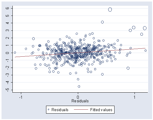
Figure 5.10, page 158.
drop yresid xresid d yhat
regress wtr81_3 inc_3 retire educat logpeop clogpeop

  Source |       SS       df       MS                  Number of obs =     496
---------+------------------------------               F(  5,   490) =   81.82
   Model |  828.012394     5  165.602479               Prob > F      =  0.0000
Residual |  991.741348   490  2.02396193               R-squared     =  0.4550
---------+------------------------------               Adj R-squared =  0.4495
   Total |  1819.75374   495  3.67627019               Root MSE      =  1.4227

------------------------------------------------------------------------------
 wtr81_3 |      Coef.   Std. Err.       t     P>|t|       [95% Conf. Interval]
---------+--------------------------------------------------------------------
   inc_3 |   1.047983   .1774549      5.906   0.000       .6993166     1.39665
  retire |  -.0673496   .1654594     -0.407   0.684      -.3924471    .2577478
  educat |  -.0387927   .0223117     -1.739   0.083      -.0826312    .0050458
 logpeop |   1.842966   .1355056     13.601   0.000       1.576722     2.10921
clogpeop |  -.0053465   .3612487     -0.015   0.988      -.7151341     .704441
   _cons |   5.949177   .4662837     12.759   0.000       5.033014    6.865339
------------------------------------------------------------------------------

predict yresid, residual
regress wtr80_3 inc_3 retire educat logpeop clogpeop

  Source |       SS       df       MS                  Number of obs =     496
---------+------------------------------               F(  5,   490) =   61.12
   Model |  768.524459     5  153.704892               Prob > F      =  0.0000
Residual |  1232.20683   490  2.51470781               R-squared     =  0.3841
---------+------------------------------               Adj R-squared =  0.3778
   Total |  2000.73129   495  4.04188139               Root MSE      =  1.5858

------------------------------------------------------------------------------
 wtr80_3 |      Coef.   Std. Err.       t     P>|t|       [95% Conf. Interval]
---------+--------------------------------------------------------------------
   inc_3 |    .850937    .197802      4.302   0.000       .4622922    1.239582
  retire |  -.2697662    .184431     -1.463   0.144      -.6321394    .0926071
  educat |  -.0042506     .02487     -0.171   0.864      -.0531157    .0446144
 logpeop |     1.8038   .1510427     11.942   0.000       1.507029    2.100572
clogpeop |  -1.472482   .4026696     -3.657   0.000      -2.263654   -.6813101
   _cons |   6.543406    .519748     12.590   0.000       5.522196    7.564615
------------------------------------------------------------------------------

predict xresid, residual
regress yresid xresid

  Source |       SS       df       MS                  Number of obs =     496
---------+------------------------------               F(  1,   494) =  467.31
   Model |    482.1047     1    482.1047               Prob > F      =  0.0000
Residual |  509.636644   494  1.03165313               R-squared     =  0.4861
---------+------------------------------               Adj R-squared =  0.4851
   Total |  991.741345   495  2.00351787               Root MSE      =  1.0157

------------------------------------------------------------------------------
  yresid |      Coef.   Std. Err.       t     P>|t|       [95% Conf. Interval]
---------+--------------------------------------------------------------------
  xresid |   .6255023   .0289351     21.617   0.000       .5686512    .6823533
   _cons |   1.10e-09   .0456064      0.000   1.000      -.0896065    .0896065
------------------------------------------------------------------------------

predict yhat
predict d, cooksd
gen cook = .
replace cook = (99/4)*d*(d+1)^2 + 1 if d <=1
replace cook = 100 if d >1
graph twoway (scatter yresid xresid [w=cook], msymbol(oh)) (lfit yresid xresid), ///
		ylabel(-5(1)5) xlabel(-5(1)5)
Page 159. Means listed at the top of the page.
summarize inc_3 wtr80_3 educat retire logpeop clogpeop

Variable |     Obs        Mean   Std. Dev.       Min        Max
---------+-----------------------------------------------------
   inc_3 |     496    2.474998   .4471152   1.231144   3.981072
 wtr80_3 |     496    10.29697   2.010443   4.901274   17.02712
  educat |     496    14.00403    3.09055          6         20
  retire |     496    .2943548   .4562123          0          1
 logpeop |     496    .9750739   .5588389          0   2.302585
clogpeop |     496   -.0187373   .1826309  -1.098612   1.386294
This gives Equation [5.14a].
regress wtr81_3 inc_3 wtr80_3 educat retire logpeop clogpeop

  Source |       SS       df       MS                  Number of obs =     496
---------+------------------------------               F(  6,   489) =  209.51
   Model |   1310.1171     6   218.35285               Prob > F      =  0.0000
Residual |  509.636644   489  1.04220173               R-squared     =  0.7199
---------+------------------------------               Adj R-squared =  0.7165
   Total |  1819.75374   495  3.67627019               Root MSE      =  1.0209

------------------------------------------------------------------------------
 wtr81_3 |      Coef.   Std. Err.       t     P>|t|       [95% Conf. Interval]
---------+--------------------------------------------------------------------
   inc_3 |     .51572   .1297219      3.976   0.000        .260839    .7706011
 wtr80_3 |   .6255023   .0290827     21.508   0.000       .5683599    .6826446
  educat |  -.0361339   .0160111     -2.257   0.024       -.067593   -.0046749
  retire |   .1013897   .1189905      0.852   0.395       -.132406    .3351855
 logpeop |   .7146849   .1104854      6.469   0.000       .4976001    .9317696
clogpeop |   .9156945   .2627408      3.485   0.001       .3994542    1.431935
   _cons |   1.856262   .3849294      4.822   0.000       1.099942    2.612581
------------------------------------------------------------------------------
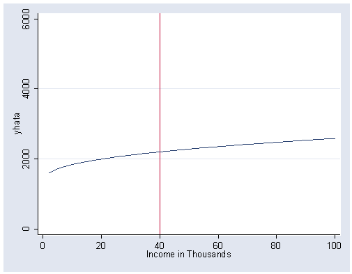
Figure 5.11, page 160.
NOTE: Use Equation [5.14b].
gen yhat1=8.507+.516*(income^.3)
gen yhata=yhat1^(1/.3)
graph twoway line yhata income, sort ylabel(1600(200)2400) xlabel(0(20)100)
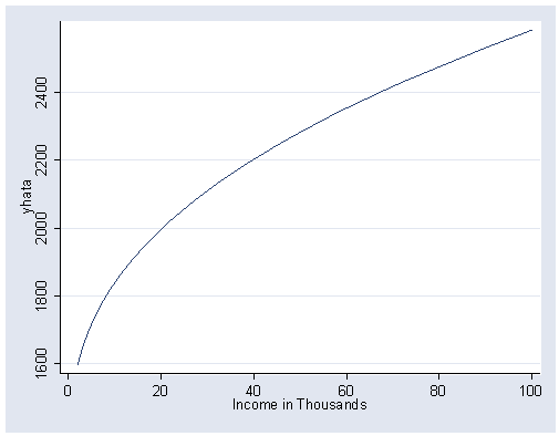
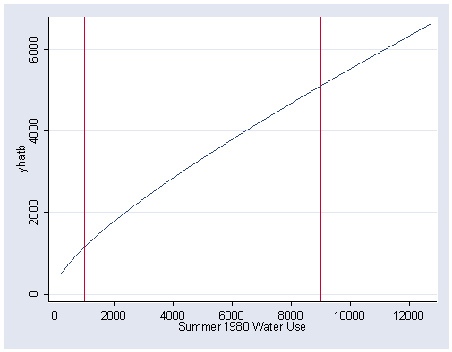
Figure 5.12, page 161.
Top curve:
drop yhat1 yhata
gen yhat2=14.046+.516*[income]^.3
gen yhatb=yhat2^(1/.3)
Middle curve:
gen yhat1=8.507+.516*[income]^.3
gen yhata=yhat1^(1/.3)
Bottom curve:
gen yhat3=4.204+.516*[income]^.3
gen yhatc=yhat3^(1/.3)
graph twoway (line yhatb income, sort) (line yhata income, sort) (line yhatc income, sort), ///
	        xlabel(0(20)100) ylabel(0(2000)10000)
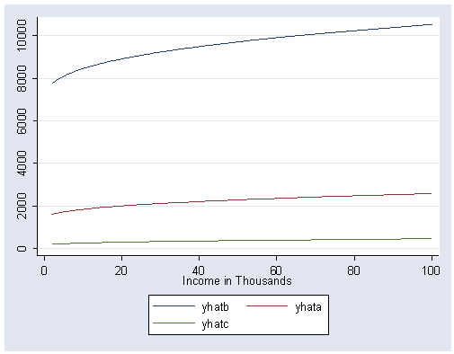
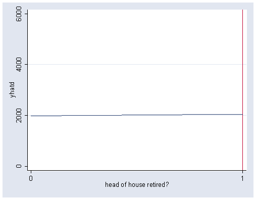
Figure 5.13, page 162.
use https://stats.idre.ucla.edu/stat/stata/examples/rwg/concord1, clear
gen yhat1=8.507+.516*(income^.3)
gen yhata=yhat1^(1/.3)
graph twoway line yhata income, sort xlabel(0(20)100) ylabel(0(2000)6000) xline(40)
gen yhat2=3.338+.626*(water80^.3)
gen yhatb=yhat2^(1/.3)
graph twoway line yhatb water80, ///
	sort xlabel(0(2000)12000) ylabel(0(2000)6000) xline(1000 9000)
gen yhat3=10.288-.036*(educat)
gen yhatc=yhat3^(1/.3)
graph twoway line yhatc educat, sort xlabel(6(2)20) ylabel(0(2000)6000) xline(11 20)
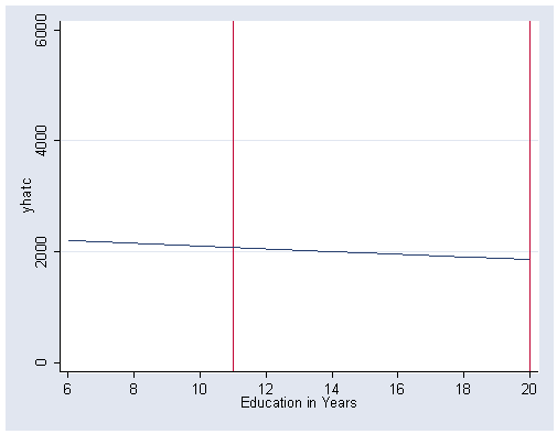
gen yhat4=9.755+.101*(retire)
gen yhatd=yhat4^(1/.3)
graph twoway line yhatd retire, sort xlabel(0 1) ylabel(0(2000)6000) xline(1)
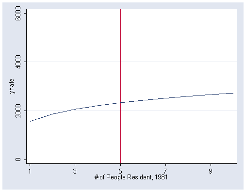
gen yhat5=9.087+.715*(ln(peop81))
gen yhate=yhat5^(1/.3)
graph twoway line yhate peop81, sort xlabel(1(2)10) ylabel(0(2000)6000) xline(5)
gen x=peop81/peop80
gen yhat6=9.802+.916*(ln(x))
gen yhatf=yhat6^(1/.3)
graph twoway line yhatf x, sort xlabel(0(1)4) ylabel(0(2000)6000) xline(1)
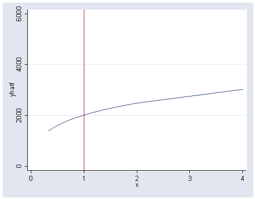
Table 5.3, page 168. The noobs option tells Stata not to display the observation number, and the nodis option puts the output in the table form used in the book.
use https://stats.idre.ucla.edu/stat/stata/examples/rwg/child, clear

list age c1920 c1930 c1940 c1945 c1950 c1955 c1960 if (c1945~=.), noobs nodis

     age     c1920     c1930     c1940     c1945     c1950     c1955     c1960
      15         0         0         0         0         0         0         0
      20         7         9        13        17        19        18        13
      25        39        48        59        60        53        45        39
      30        67        75        82        82        75        68         .
      35        76        83        87        88        83         .         .
      40        78        86        89        90         .         .         .
Table 5.4, page 169.
Note: Because of differences in the algorithms used by the version of Stata used when creating this table and version 6, fewer iterations are needed to produce the same results. The eps option is forcing Stata to do three more iterations than it would do without the option. Despite the difference in algorithms, the results are the same.
Note that gomh is an .ado program that you need to run before you can use the nl gomh command. The gomh program defines the equation shown at the top of Table 5.4.
program define nlgomh
  version 6.0
  if "`1'"  == "?" {
  global S_1  "Alpha Gamma Beta"
  global Alpha = 89
  global Gamma = 942
  global Beta = 0.31
  exit
 }
replace `1' = $Alpha * exp(-1* $Gamma * exp(-1*$Beta*age))
end

nl gomh c1945, eps(0.00000000001) trace
(obs = 6)

Iteration 0:
           Alpha =        89
           Gamma =       942
           Beta =       .31
                                         residual SS =  17.54198
Iteration 1:
           Alpha =  89.69356
           Gamma =  589.8155
           Beta =  .2948988
                                         residual SS =  4.928977
Iteration 2:
           Alpha =  90.39808
           Gamma =  443.0836
           Beta =  .2808511
                                         residual SS =  1.970012
Iteration 3:
           Alpha =  90.42829
           Gamma =  465.8808
           Beta =  .2815535
                                         residual SS =  .1213906
Iteration 4:
           Alpha =  90.42532
           Gamma =   468.054
           Beta =  .2817029
                                         residual SS =  .1184228
Iteration 5:
           Alpha =  90.42534
           Gamma =  468.0575
           Beta =  .2817027
                                         residual SS =  .1184227
Iteration 6:
           Alpha =  90.42534
           Gamma =  468.0575
           Beta =  .2817027
                                         residual SS =  .1184227
Iteration 7:
           Alpha =  90.42534
           Gamma =  468.0575
           Beta =  .2817027
                                         residual SS =  .1184227


  Source |       SS       df       MS                Number of obs =         6
---------+------------------------------             F(  3,     3) = 223410.65
   Model |  26456.8816     3  8818.96053             Prob > F      =    0.0000
Residual |   .11842265     3  .039474217             R-squared     =    1.0000
---------+------------------------------             Adj R-squared =    1.0000
   Total |       26457     6      4409.5             Root MSE      =  .1986812
                                                     Res. dev.     = -6.524266
(gomh)
------------------------------------------------------------------------------
   c1945 |      Coef.   Std. Err.       t     P>|t|       [95% Conf. Interval]
---------+--------------------------------------------------------------------
   Alpha |   90.42534    .160669    562.805   0.000       89.91402    90.93666
   Gamma |   468.0575   22.54659     20.760   0.000       396.3042    539.8108
    Beta |   .2817027   .0022184    126.982   0.000       .2746427    .2887628
------------------------------------------------------------------------------
 (SE's, P values, CI's, and correlations are asymptotic approximations)
Figure 5.19, page 169.
predict y
graph twoway (line y age, sort) (scatter c1945 age), ylabel(0(10)90) xlabel(15(5)40)
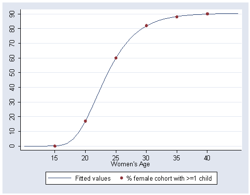
Table 5.5, page 170.
nl gomh c1945, iter(10)
(obs = 6)

Iteration 0:  residual SS =  17.54198
Iteration 1:  residual SS =  4.928977
Iteration 2:  residual SS =  1.970012
Iteration 3:  residual SS =  .1213906
Iteration 4:  residual SS =  .1184228

  Source |       SS       df       MS                Number of obs =         6
---------+------------------------------             F(  3,     3) = 223410.65
   Model |  26456.8816     3  8818.96053             Prob > F      =    0.0000
Residual |   .11842265     3  .039474217             R-squared     =    1.0000
---------+------------------------------             Adj R-squared =    1.0000
   Total |       26457     6      4409.5             Root MSE      =  .1986812
                                                     Res. dev.     = -6.524266
(gomh)
------------------------------------------------------------------------------
   c1945 |      Coef.   Std. Err.       t     P>|t|       [95% Conf. Interval]
---------+--------------------------------------------------------------------
   Alpha |   90.42534   .1606687    562.806   0.000       89.91402    90.93666
   Gamma |   468.0575   22.54646     20.760   0.000       396.3046    539.8104
    Beta |   .2817027   .0022185    126.982   0.000       .2746426    .2887629
------------------------------------------------------------------------------
 (SE's, P values, CI's, and correlations are asymptotic approximations)

predict r, resid
(31 missing values generated)

summarize r, detail

                         Residuals
-------------------------------------------------------------
      Percentiles      Smallest
 1%    -.2409922      -.2409922
 5%    -.2409922      -.0965911
10%    -.2409922      -.0693029       Obs                   6
25%    -.0965911        .026351       Sum of Wgt.           6

50%    -.0214759                      Mean          -.0143851
                        Largest       Std. Dev.      .1530889
75%     .1136894      -.0693029
90%     .1805354        .026351       Variance       .0234362
95%     .1805354       .1136894       Skewness      -.1699677
99%     .1805354       .1805354       Kurtosis        1.92567

* Stata 8 code.
vce, rho

* Stata 9 code and output.
estat vce, rho

Correlation matrix of coefficients of nl model

        e(V) |    Alpha     Gamma      Beta
-------------+------------------------------
       Alpha |   1.0000
       Gamma |  -0.5869    1.0000
        Beta |  -0.6342    0.9927    1.0000
Table 5.6, page 172.
nl gomh c1920 c1930 c1940 c1945 c1950 c1955
(obs = 4)

Iteration 0:  residual SS =  665.4337
Iteration 1:  residual SS =   492.565
Iteration 2:  residual SS =  460.7865
Iteration 3:  residual SS =  191.9489
Iteration 4:  residual SS =  6.350819
Iteration 5:  residual SS =  1.521302
Iteration 6:  residual SS =  .7325416
Iteration 7:  residual SS =  .2211592
Iteration 8:  residual SS =  .0009551
Iteration 9:  residual SS =  .0008995

  Source |       SS       df       MS                Number of obs =         4
---------+------------------------------             F(  3,     1) = 2245269.07
   Model |   6058.9991     3  2019.66637             Prob > F      =    0.0005
Residual |  .000899521     1  .000899521             R-squared     =    1.0000
---------+------------------------------             Adj R-squared =    1.0000
   Total |        6059     4     1514.75             Root MSE      =   .029992
                                                     Res. dev.     = -22.24826
(gomh)
------------------------------------------------------------------------------
   c1920 |      Coef.   Std. Err.       t     P>|t|       [95% Conf. Interval]
---------+--------------------------------------------------------------------
   Alpha |   85.93022   .1436735    598.094   0.001       84.10467    87.75576
   Gamma |   254.6832   3.478409     73.218   0.009       210.4859    298.8806
    Beta |   .2310315   .0006446    358.393   0.002       .2228407    .2392224
------------------------------------------------------------------------------
 (SE's, P values, CI's, and correlations are asymptotic approximations)
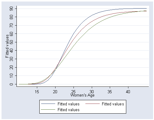
Figure 5.20, page 172.
nl gom3 c1945 age, init(b1=90.4, b2=.28, b3=25.312)
(obs = 6)

Iteration 0:  residual SS =  1312.106
Iteration 1:  residual SS =  183.3323
Iteration 2:  residual SS =  52.10777
Iteration 3:  residual SS =  .2411037
Iteration 4:  residual SS =  .1184235
Iteration 5:  residual SS =  .1184227

  Source |       SS       df       MS                Number of obs =         6
---------+------------------------------             F(  3,     3) = 223410.65
   Model |  26456.8816     3  8818.96053             Prob > F      =    0.0000
Residual |   .11842265     3  .039474217             R-squared     =    1.0000
---------+------------------------------             Adj R-squared =    1.0000
   Total |       26457     6      4409.5             Root MSE      =  .1986812
                                                     Res. dev.     = -6.524266
3-parameter Gompertz function, c1945=b1*exp(-exp(-b2*(age-b3)))
------------------------------------------------------------------------------
   c1945 |      Coef.   Std. Err.       t     P>|t|       [95% Conf. Interval]
---------+--------------------------------------------------------------------
      b1 |   90.42534   .1606689    562.806   0.000       89.91402    90.93666
      b2 |   .2817027   .0022184    126.983   0.000       .2746427    .2887628
      b3 |   21.82652   .0207139   1053.713   0.000        21.7606    21.89244
------------------------------------------------------------------------------
 (SE's, P values, CI's, and correlations are asymptotic approximations)

predict a, yhat
nl gom3 c1950 age, init(b1=87.5, b2=.23, b3=20.125)
(obs = 5)

Iteration 0:  residual SS =  283.4875
Iteration 1:  residual SS =  5.771125
Iteration 2:  residual SS =  .8891598
Iteration 3:  residual SS =  .8549497
Iteration 4:  residual SS =  .8549349
Iteration 5:  residual SS =  .8549348

  Source |       SS       df       MS                Number of obs =         5
---------+------------------------------             F(  3,     2) =  12229.51
   Model |  15683.1451     3  5227.71502             Prob > F      =    0.0001
Residual |  .854934809     2  .427467404             R-squared     =    0.9999
---------+------------------------------             Adj R-squared =    0.9999
   Total |       15684     5      3136.8             Root MSE      =  .6538099
                                                     Res. dev.     =  5.358545
3-parameter Gompertz function, c1950=b1*exp(-exp(-b2*(age-b3)))
------------------------------------------------------------------------------
   c1950 |      Coef.   Std. Err.       t     P>|t|       [95% Conf. Interval]
---------+--------------------------------------------------------------------
      b1 |    87.5145   1.021152     85.702   0.000       83.12084    91.90816
      b2 |   .2271519   .0080141     28.344   0.001       .1926701    .2616337
      b3 |    21.9059   .0975443    224.574   0.000       21.48621     22.3256
------------------------------------------------------------------------------
 (SE's, P values, CI's, and correlations are asymptotic approximations)

predict b, yhat
nl gom3 c1955 age, init(b1=88.9, b2=.18, b3=16.002)
(obs = 4)

Iteration 0:  residual SS =  3039.062
Iteration 1:  residual SS =   1012.67
Iteration 2:  residual SS =  947.3681
Iteration 3:  residual SS =  818.6254
Iteration 4:  residual SS =  395.6796
Iteration 5:  residual SS =    200.15
Iteration 6:  residual SS =  35.09833
Iteration 7:  residual SS =  4.517478
Iteration 8:  residual SS =  3.492366
Iteration 9:  residual SS =  3.489542
Iteration 10:  residual SS =  3.489428
Iteration 11:  residual SS =  3.489423
Iteration 12:  residual SS =  3.489423
Iteration 13:  residual SS =  3.489423

  Source |       SS       df       MS                Number of obs =         4
---------+------------------------------             F(  3,     1) =    665.77
   Model |  6969.51058     3  2323.17019             Prob > F      =    0.0285
Residual |  3.48942272     1  3.48942272             R-squared     =    0.9995
---------+------------------------------             Adj R-squared =    0.9980
   Total |        6973     4     1743.25             Root MSE      =     1.868
                                                     Res. dev.     =  10.80528
3-parameter Gompertz function, c1955=b1*exp(-exp(-b2*(age-b3)))
------------------------------------------------------------------------------
   c1955 |      Coef.   Std. Err.       t     P>|t|       [95% Conf. Interval]
---------+--------------------------------------------------------------------
      b1 |   88.94686   10.49314      8.477   0.075      -44.38107    222.2748
      b2 |   .1800778    .033323      5.404   0.116       -.243331    .6034866
      b3 |   22.76404   .8402734     27.091   0.023       12.08735    33.44073
------------------------------------------------------------------------------
 (SE's, P values, CI's, and correlations are asymptotic approximations)

predict c, yhat
graph twoway (line a age, sort) (line b age, sort) (line c age, sort), ///
	        ylabel(0(10)90) xlabel(15(5)40)