Everything? No, that’s a gross exaggeration. If you want to know everything about contrasts you will need read several other sources in addition to this page. Here are our suggestions:
Mitchell, M.N. 2012. Interpreting and Visualizing Regression Models Using Stata. College Station, TX: Stata Press. StataCorp. 2009. Stata 11 Base Reference Manual. College Station, TX: Stata Press. Topics: contrast, margins, margins, comtrast, margins, pwcompare, marginsplot and pwcompare.
This page will cover a lot of examples without a lot of verbiage. But first, one more thing.
What is a contrast?
A contrast is a one degree of freedom test comparing means. One degree of freedom? You mean I can only compare two means? No, you can compare more than two means if you do it correctly. For example, you can compare the average of the means of groups 1 and 2 versus the mean of group 3. This contrast involves three means but uses only one degree of freedom.
Let’s begin.
One-factor Model
We will begin with a one-factor model with four levels. First, we will load the data run the model, get the cell means and plot them. We can run the model using either anova or regress. Either way we will get the same results. We will use the anova command this time.
use https://stats.idre.ucla.edu/stat/data/hsbanova, clear
anova write grp
Number of obs = 200 R-squared = 0.1939
Root MSE = 8.5752 Adj R-squared = 0.1815
Source | Partial SS df MS F Prob > F
-----------+----------------------------------------------------
Model | 3466.19389 3 1155.39796 15.71 0.0000
|
grp | 3466.19389 3 1155.39796 15.71 0.0000
|
Residual | 14412.6811 196 73.5340873
-----------+----------------------------------------------------
Total | 17878.875 199 89.843593
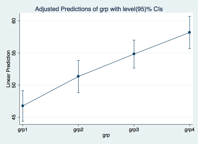
margins grp // get cell means
Adjusted predictions Number of obs = 200
Expression : Linear prediction, predict()
------------------------------------------------------------------------------
| Delta-method
| Margin Std. Err. z P>|z| [95% Conf. Interval]
-------------+----------------------------------------------------------------
grp |
1 | 46.76 1.212717 38.56 0.000 44.38312 49.13688
2 | 51.33333 1.278316 40.16 0.000 48.82788 53.83879
3 | 54.81667 1.107054 49.52 0.000 52.64688 56.98645
4 | 58.17778 1.278316 45.51 0.000 55.67233 60.68323
------------------------------------------------------------------------------
marginsplot
 * Reference group contrast
contrast r.grp, effects
Contrasts of marginal linear predictions
Margins : asbalanced
------------------------------------------------
| df F P>F
-------------+----------------------------------
grp |
(2 vs 1) | 1 6.74 0.0102
(3 vs 1) | 1 24.07 0.0000
(4 vs 1) | 1 41.99 0.0000
Joint | 3 15.71 0.0000
|
Residual | 196
------------------------------------------------
------------------------------------------------------------------------------
| Contrast Std. Err. t P>|t| [95% Conf. Interval]
-------------+----------------------------------------------------------------
grp |
(2 vs 1) | 4.573333 1.762036 2.60 0.010 1.098349 8.048318
(3 vs 1) | 8.056667 1.642026 4.91 0.000 4.818359 11.29497
(4 vs 1) | 11.41778 1.762036 6.48 0.000 7.942793 14.89276
------------------------------------------------------------------------------
* Change the reference group to grp3.
contrast rb3.grp, effects // change reference group to grp3
Contrasts of marginal linear predictions
Margins : asbalanced
------------------------------------------------
| df F P>F
-------------+----------------------------------
grp |
(1 vs 3) | 1 24.07 0.0000
(2 vs 3) | 1 4.24 0.0407
(4 vs 3) | 1 3.95 0.0482
Joint | 3 15.71 0.0000
|
Residual | 196
------------------------------------------------
------------------------------------------------------------------------------
| Contrast Std. Err. t P>|t| [95% Conf. Interval]
-------------+----------------------------------------------------------------
grp |
(1 vs 3) | -8.056667 1.642026 -4.91 0.000 -11.29497 -4.818359
(2 vs 3) | -3.483333 1.691053 -2.06 0.041 -6.818328 -.1483388
(4 vs 3) | 3.361111 1.691053 1.99 0.048 .0261165 6.696106
------------------------------------------------------------------------------
* Adjacent group contrast
contrast a.grp, effects
Contrasts of marginal linear predictions
Margins : asbalanced
------------------------------------------------
| df F P>F
-------------+----------------------------------
grp |
(1 vs 2) | 1 6.74 0.0102
(2 vs 3) | 1 4.24 0.0407
(3 vs 4) | 1 3.95 0.0482
Joint | 3 15.71 0.0000
|
Residual | 196
------------------------------------------------
------------------------------------------------------------------------------
| Contrast Std. Err. t P>|t| [95% Conf. Interval]
-------------+----------------------------------------------------------------
grp |
(1 vs 2) | -4.573333 1.762036 -2.60 0.010 -8.048318 -1.098349
(2 vs 3) | -3.483333 1.691053 -2.06 0.041 -6.818328 -.1483388
(3 vs 4) | -3.361111 1.691053 -1.99 0.048 -6.696106 -.0261165
------------------------------------------------------------------------------
* Grand mean contrast
contrast g.grp, effects
Contrasts of marginal linear predictions
Margins : asbalanced
------------------------------------------------
| df F P>F
-------------+----------------------------------
grp |
(1 vs mean) | 1 32.62 0.0000
(2 vs mean) | 1 1.74 0.1888
(3 vs mean) | 1 4.24 0.0408
(4 vs mean) | 1 24.56 0.0000
Joint | 3 15.71 0.0000
|
Residual | 196
------------------------------------------------
------------------------------------------------------------------------------
| Contrast Std. Err. t P>|t| [95% Conf. Interval]
-------------+----------------------------------------------------------------
grp |
(1 vs mean) | -6.011944 1.052672 -5.71 0.000 -8.087962 -3.935927
(2 vs mean) | -1.438611 1.09079 -1.32 0.189 -3.589803 .7125804
(3 vs mean) | 2.044722 .9927543 2.06 0.041 .0868706 4.002574
(4 vs mean) | 5.405833 1.09079 4.96 0.000 3.254642 7.557025
------------------------------------------------------------------------------
* Helmert contrast
contrast h.grp, effects
Contrasts of marginal linear predictions
Margins : asbalanced
------------------------------------------------
| df F P>F
-------------+----------------------------------
grp |
(1 vs >1) | 1 32.62 0.0000
(2 vs >2) | 1 11.35 0.0009
(3 vs 4) | 1 3.95 0.0482
Joint | 3 15.71 0.0000
|
Residual | 196
------------------------------------------------
------------------------------------------------------------------------------
| Contrast Std. Err. t P>|t| [95% Conf. Interval]
-------------+----------------------------------------------------------------
grp |
(1 vs >1) | -8.015926 1.403562 -5.71 0.000 -10.78395 -5.247903
(2 vs >2) | -5.163889 1.532647 -3.37 0.001 -8.186484 -2.141293
(3 vs 4) | -3.361111 1.691053 -1.99 0.048 -6.696106 -.0261165
------------------------------------------------------------------------------
* Polynomial contrast
contrast p.grp, effects
Contrasts of marginal linear predictions
Margins : asbalanced
------------------------------------------------
| df F P>F
-------------+----------------------------------
grp |
(linear) | 1 46.23 0.0000
(quadratic) | 1 0.25 0.6202
(cubic) | 1 0.03 0.8572
Joint | 3 15.71 0.0000
|
Residual | 196
------------------------------------------------
------------------------------------------------------------------------------
| Contrast Std. Err. t P>|t| [95% Conf. Interval]
-------------+----------------------------------------------------------------
grp |
(linear) | 4.219088 .62051 6.80 0.000 2.995354 5.442821
(quadratic) | -.3030556 .6105546 -0.50 0.620 -1.507156 .9010444
(cubic) | .1082008 .6004343 0.18 0.857 -1.07594 1.292342
------------------------------------------------------------------------------
* User defined contrast grp1 vs grp4
contrast {grp 1 0 0 -1}, effects
Contrasts of marginal linear predictions
Margins : asbalanced
------------------------------------------------
| df F P>F
-------------+----------------------------------
grp | 1 41.99 0.0000
|
Residual | 196
------------------------------------------------
------------------------------------------------------------------------------
| Contrast Std. Err. t P>|t| [95% Conf. Interval]
-------------+----------------------------------------------------------------
grp |
(1) | -11.41778 1.762036 -6.48 0.000 -14.89276 -7.942793
------------------------------------------------------------------------------
* Nonpairwise user defined contrast, grp2 vs average of grp3 & grp4
contrast {grp 0 1 -.5 -.5}, effects // nonpairwise contrast
Contrasts of marginal linear predictions
Margins : asbalanced
------------------------------------------------
| df F P>F
-------------+----------------------------------
grp | 1 11.35 0.0009
|
Residual | 196
------------------------------------------------
------------------------------------------------------------------------------
| Contrast Std. Err. t P>|t| [95% Conf. Interval]
-------------+----------------------------------------------------------------
grp |
(1) | -5.163889 1.532647 -3.37 0.001 -8.186484 -2.141293
------------------------------------------------------------------------------
* All pairwise comparisons with Tukey adjustment
pwcompare grp, mcompare(tukey) effects group
Pairwise comparisons of marginal linear predictions
Margins : asbalanced
---------------------------
| Number of
| Comparisons
-------------+-------------
grp | 6
---------------------------
----------------------------------------------
| Tukey
| Margin Std. Err. Groups
-------------+--------------------------------
grp |
1 | 46.76 1.212717
2 | 51.33333 1.278316 A
3 | 54.81667 1.107054 AB
4 | 58.17778 1.278316 B
----------------------------------------------
Note: Margins sharing a letter in the group
label are not significantly different at
the 5% level.
Note: The tukey method requires balanced data
for proper level coverage. A factor was
found to be unbalanced.
---------------------------
| Number of
| Comparisons
-------------+-------------
grp | 6
---------------------------
------------------------------------------------------------------------------
| Tukey Tukey
| Contrast Std. Err. t P>|t| [95% Conf. Interval]
-------------+----------------------------------------------------------------
grp |
2 vs 1 | 4.573333 1.762036 2.60 0.049 .0075312 9.139136
3 vs 1 | 8.056667 1.642026 4.91 0.000 3.801836 12.3115
4 vs 1 | 11.41778 1.762036 6.48 0.000 6.851976 15.98358
3 vs 2 | 3.483333 1.691053 2.06 0.170 -.8985349 7.865202
4 vs 2 | 6.844444 1.807811 3.79 0.001 2.16003 11.52886
4 vs 3 | 3.361111 1.691053 1.99 0.196 -1.020757 7.742979
------------------------------------------------------------------------------
Note: The tukey method requires balanced data for proper level coverage. A
factor was found to be unbalanced.
* Reference group contrast
contrast r.grp, effects
Contrasts of marginal linear predictions
Margins : asbalanced
------------------------------------------------
| df F P>F
-------------+----------------------------------
grp |
(2 vs 1) | 1 6.74 0.0102
(3 vs 1) | 1 24.07 0.0000
(4 vs 1) | 1 41.99 0.0000
Joint | 3 15.71 0.0000
|
Residual | 196
------------------------------------------------
------------------------------------------------------------------------------
| Contrast Std. Err. t P>|t| [95% Conf. Interval]
-------------+----------------------------------------------------------------
grp |
(2 vs 1) | 4.573333 1.762036 2.60 0.010 1.098349 8.048318
(3 vs 1) | 8.056667 1.642026 4.91 0.000 4.818359 11.29497
(4 vs 1) | 11.41778 1.762036 6.48 0.000 7.942793 14.89276
------------------------------------------------------------------------------
* Change the reference group to grp3.
contrast rb3.grp, effects // change reference group to grp3
Contrasts of marginal linear predictions
Margins : asbalanced
------------------------------------------------
| df F P>F
-------------+----------------------------------
grp |
(1 vs 3) | 1 24.07 0.0000
(2 vs 3) | 1 4.24 0.0407
(4 vs 3) | 1 3.95 0.0482
Joint | 3 15.71 0.0000
|
Residual | 196
------------------------------------------------
------------------------------------------------------------------------------
| Contrast Std. Err. t P>|t| [95% Conf. Interval]
-------------+----------------------------------------------------------------
grp |
(1 vs 3) | -8.056667 1.642026 -4.91 0.000 -11.29497 -4.818359
(2 vs 3) | -3.483333 1.691053 -2.06 0.041 -6.818328 -.1483388
(4 vs 3) | 3.361111 1.691053 1.99 0.048 .0261165 6.696106
------------------------------------------------------------------------------
* Adjacent group contrast
contrast a.grp, effects
Contrasts of marginal linear predictions
Margins : asbalanced
------------------------------------------------
| df F P>F
-------------+----------------------------------
grp |
(1 vs 2) | 1 6.74 0.0102
(2 vs 3) | 1 4.24 0.0407
(3 vs 4) | 1 3.95 0.0482
Joint | 3 15.71 0.0000
|
Residual | 196
------------------------------------------------
------------------------------------------------------------------------------
| Contrast Std. Err. t P>|t| [95% Conf. Interval]
-------------+----------------------------------------------------------------
grp |
(1 vs 2) | -4.573333 1.762036 -2.60 0.010 -8.048318 -1.098349
(2 vs 3) | -3.483333 1.691053 -2.06 0.041 -6.818328 -.1483388
(3 vs 4) | -3.361111 1.691053 -1.99 0.048 -6.696106 -.0261165
------------------------------------------------------------------------------
* Grand mean contrast
contrast g.grp, effects
Contrasts of marginal linear predictions
Margins : asbalanced
------------------------------------------------
| df F P>F
-------------+----------------------------------
grp |
(1 vs mean) | 1 32.62 0.0000
(2 vs mean) | 1 1.74 0.1888
(3 vs mean) | 1 4.24 0.0408
(4 vs mean) | 1 24.56 0.0000
Joint | 3 15.71 0.0000
|
Residual | 196
------------------------------------------------
------------------------------------------------------------------------------
| Contrast Std. Err. t P>|t| [95% Conf. Interval]
-------------+----------------------------------------------------------------
grp |
(1 vs mean) | -6.011944 1.052672 -5.71 0.000 -8.087962 -3.935927
(2 vs mean) | -1.438611 1.09079 -1.32 0.189 -3.589803 .7125804
(3 vs mean) | 2.044722 .9927543 2.06 0.041 .0868706 4.002574
(4 vs mean) | 5.405833 1.09079 4.96 0.000 3.254642 7.557025
------------------------------------------------------------------------------
* Helmert contrast
contrast h.grp, effects
Contrasts of marginal linear predictions
Margins : asbalanced
------------------------------------------------
| df F P>F
-------------+----------------------------------
grp |
(1 vs >1) | 1 32.62 0.0000
(2 vs >2) | 1 11.35 0.0009
(3 vs 4) | 1 3.95 0.0482
Joint | 3 15.71 0.0000
|
Residual | 196
------------------------------------------------
------------------------------------------------------------------------------
| Contrast Std. Err. t P>|t| [95% Conf. Interval]
-------------+----------------------------------------------------------------
grp |
(1 vs >1) | -8.015926 1.403562 -5.71 0.000 -10.78395 -5.247903
(2 vs >2) | -5.163889 1.532647 -3.37 0.001 -8.186484 -2.141293
(3 vs 4) | -3.361111 1.691053 -1.99 0.048 -6.696106 -.0261165
------------------------------------------------------------------------------
* Polynomial contrast
contrast p.grp, effects
Contrasts of marginal linear predictions
Margins : asbalanced
------------------------------------------------
| df F P>F
-------------+----------------------------------
grp |
(linear) | 1 46.23 0.0000
(quadratic) | 1 0.25 0.6202
(cubic) | 1 0.03 0.8572
Joint | 3 15.71 0.0000
|
Residual | 196
------------------------------------------------
------------------------------------------------------------------------------
| Contrast Std. Err. t P>|t| [95% Conf. Interval]
-------------+----------------------------------------------------------------
grp |
(linear) | 4.219088 .62051 6.80 0.000 2.995354 5.442821
(quadratic) | -.3030556 .6105546 -0.50 0.620 -1.507156 .9010444
(cubic) | .1082008 .6004343 0.18 0.857 -1.07594 1.292342
------------------------------------------------------------------------------
* User defined contrast grp1 vs grp4
contrast {grp 1 0 0 -1}, effects
Contrasts of marginal linear predictions
Margins : asbalanced
------------------------------------------------
| df F P>F
-------------+----------------------------------
grp | 1 41.99 0.0000
|
Residual | 196
------------------------------------------------
------------------------------------------------------------------------------
| Contrast Std. Err. t P>|t| [95% Conf. Interval]
-------------+----------------------------------------------------------------
grp |
(1) | -11.41778 1.762036 -6.48 0.000 -14.89276 -7.942793
------------------------------------------------------------------------------
* Nonpairwise user defined contrast, grp2 vs average of grp3 & grp4
contrast {grp 0 1 -.5 -.5}, effects // nonpairwise contrast
Contrasts of marginal linear predictions
Margins : asbalanced
------------------------------------------------
| df F P>F
-------------+----------------------------------
grp | 1 11.35 0.0009
|
Residual | 196
------------------------------------------------
------------------------------------------------------------------------------
| Contrast Std. Err. t P>|t| [95% Conf. Interval]
-------------+----------------------------------------------------------------
grp |
(1) | -5.163889 1.532647 -3.37 0.001 -8.186484 -2.141293
------------------------------------------------------------------------------
* All pairwise comparisons with Tukey adjustment
pwcompare grp, mcompare(tukey) effects group
Pairwise comparisons of marginal linear predictions
Margins : asbalanced
---------------------------
| Number of
| Comparisons
-------------+-------------
grp | 6
---------------------------
----------------------------------------------
| Tukey
| Margin Std. Err. Groups
-------------+--------------------------------
grp |
1 | 46.76 1.212717
2 | 51.33333 1.278316 A
3 | 54.81667 1.107054 AB
4 | 58.17778 1.278316 B
----------------------------------------------
Note: Margins sharing a letter in the group
label are not significantly different at
the 5% level.
Note: The tukey method requires balanced data
for proper level coverage. A factor was
found to be unbalanced.
---------------------------
| Number of
| Comparisons
-------------+-------------
grp | 6
---------------------------
------------------------------------------------------------------------------
| Tukey Tukey
| Contrast Std. Err. t P>|t| [95% Conf. Interval]
-------------+----------------------------------------------------------------
grp |
2 vs 1 | 4.573333 1.762036 2.60 0.049 .0075312 9.139136
3 vs 1 | 8.056667 1.642026 4.91 0.000 3.801836 12.3115
4 vs 1 | 11.41778 1.762036 6.48 0.000 6.851976 15.98358
3 vs 2 | 3.483333 1.691053 2.06 0.170 -.8985349 7.865202
4 vs 2 | 6.844444 1.807811 3.79 0.001 2.16003 11.52886
4 vs 3 | 3.361111 1.691053 1.99 0.196 -1.020757 7.742979
------------------------------------------------------------------------------
Note: The tukey method requires balanced data for proper level coverage. A
factor was found to be unbalanced.
Two-factor Model
We again load the data and run the regression model this time.
use https://stats.idre.ucla.edu/stat/data/hsbanova, clear
regress write grp##female
Source | SS df MS Number of obs = 200
-------------+------------------------------ F( 7, 192) = 11.05
Model | 5135.17494 7 733.59642 Prob > F = 0.0000
Residual | 12743.7001 192 66.3734378 R-squared = 0.2872
-------------+------------------------------ Adj R-squared = 0.2612
Total | 17878.875 199 89.843593 Root MSE = 8.147
------------------------------------------------------------------------------
write | Coef. Std. Err. t P>|t| [95% Conf. Interval]
-------------+----------------------------------------------------------------
grp |
2 | 7.31677 2.458951 2.98 0.003 2.466743 12.1668
3 | 10.10248 2.292658 4.41 0.000 5.580454 14.62452
4 | 16.75286 2.525696 6.63 0.000 11.77119 21.73453
|
1.female | 9.136876 2.311726 3.95 0.000 4.577236 13.69652
|
grp#female |
2 1 | -5.029733 3.357123 -1.50 0.136 -11.65131 1.591845
3 1 | -3.721697 3.128694 -1.19 0.236 -9.892723 2.449328
4 1 | -9.831208 3.374943 -2.91 0.004 -16.48793 -3.174482
|
_cons | 41.82609 1.698765 24.62 0.000 38.47545 45.17672
------------------------------------------------------------------------------
* Test interaction and main effects
contrast grp##female
Contrasts of marginal linear predictions
Margins : asbalanced
------------------------------------------------
| df F P>F
-------------+----------------------------------
grp | 3 18.29 0.0000
|
female | 1 14.83 0.0002
|
grp#female | 3 2.89 0.0367
|
Residual | 192
------------------------------------------------
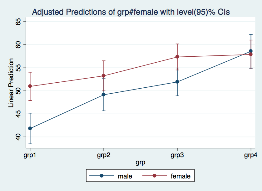
* Cell means for all 8 cells
margins grp#female
Adjusted predictions Number of obs = 200
Expression : Linear prediction, predict()
------------------------------------------------------------------------------
| Delta-method
| Margin Std. Err. z P>|z| [95% Conf. Interval]
-------------+----------------------------------------------------------------
grp#female |
1 0 | 41.82609 1.698765 24.62 0.000 38.49657 45.1556
1 1 | 50.96296 1.567889 32.50 0.000 47.88996 54.03597
2 0 | 49.14286 1.777819 27.64 0.000 45.6584 52.62732
2 1 | 53.25 1.662997 32.02 0.000 49.99059 56.50941
3 0 | 51.92857 1.539636 33.73 0.000 48.91094 54.9462
3 1 | 57.34375 1.440198 39.82 0.000 54.52101 60.16649
4 0 | 58.57895 1.869048 31.34 0.000 54.91568 62.24221
4 1 | 57.88462 1.597756 36.23 0.000 54.75307 61.01616
------------------------------------------------------------------------------
* Plot cell means
marginsplot
 * Simple contrasts & simple effects
* Simple contrasts
contrast r.grp@female, effects
Contrasts of marginal linear predictions
Margins : asbalanced
------------------------------------------------
| df F P>F
-------------+----------------------------------
grp@female |
(2 vs 1) 0 | 1 8.85 0.0033
(2 vs 1) 1 | 1 1.00 0.3183
(3 vs 1) 0 | 1 19.42 0.0000
(3 vs 1) 1 | 1 8.98 0.0031
(4 vs 1) 0 | 1 44.00 0.0000
(4 vs 1) 1 | 1 9.56 0.0023
Joint | 6 9.94 0.0000
|
Residual | 192
------------------------------------------------
------------------------------------------------------------------------------
| Contrast Std. Err. t P>|t| [95% Conf. Interval]
-------------+----------------------------------------------------------------
grp@female |
(2 vs 1) 0 | 7.31677 2.458951 2.98 0.003 2.466743 12.1668
(2 vs 1) 1 | 2.287037 2.285571 1.00 0.318 -2.221015 6.79509
(3 vs 1) 0 | 10.10248 2.292658 4.41 0.000 5.580454 14.62452
(3 vs 1) 1 | 6.380787 2.128954 3.00 0.003 2.181646 10.57993
(4 vs 1) 0 | 16.75286 2.525696 6.63 0.000 11.77119 21.73453
(4 vs 1) 1 | 6.921652 2.238549 3.09 0.002 2.506347 11.33696
------------------------------------------------------------------------------
* Simple effects
contrast grp@female
Contrasts of marginal linear predictions
Margins : asbalanced
------------------------------------------------
| df F P>F
-------------+----------------------------------
grp@female |
0 | 3 15.33 0.0000
1 | 3 4.55 0.0042
Joint | 6 9.94 0.0000
|
Residual | 192
------------------------------------------------
* Partial interactions
contrast female#a.grp
Contrasts of marginal linear predictions
Margins : asbalanced
-----------------------------------------------------
| df F P>F
------------------+----------------------------------
female#grp |
(joint) (1 vs 2) | 1 2.24 0.1357
(joint) (2 vs 3) | 1 0.16 0.6851
(joint) (3 vs 4) | 1 3.56 0.0608
Joint | 3 2.89 0.0367
|
Residual | 192
-----------------------------------------------------
* User defined contrast, female by grp1 vs grp4
contrast female#{grp 1 0 0 -1}
Contrasts of marginal linear predictions
Margins : asbalanced
------------------------------------------------
| df F P>F
-------------+----------------------------------
female#grp | 1 8.49 0.0040
|
Residual | 192
------------------------------------------------
* Treatment contrast interaction
contrast r.female#r.grp, effects
Contrasts of marginal linear predictions
Margins : asbalanced
------------------------------------------------------
| df F P>F
-------------------+----------------------------------
female#grp |
(1 vs 0) (2 vs 1) | 1 2.24 0.1357
(1 vs 0) (3 vs 1) | 1 1.41 0.2357
(1 vs 0) (4 vs 1) | 1 8.49 0.0040
Joint | 3 2.89 0.0367
|
Residual | 192
------------------------------------------------------
------------------------------------------------------------------------------
| Contrast Std. Err. t P>|t| [95% Conf. Interval]
-------------+----------------------------------------------------------------
female#grp |
(1 vs 0) |
(2 vs 1) | -5.029733 3.357123 -1.50 0.136 -11.65131 1.591845
(1 vs 0) |
(3 vs 1) | -3.721697 3.128694 -1.19 0.236 -9.892723 2.449328
(1 vs 0) |
(4 vs 1) | -9.831208 3.374943 -2.91 0.004 -16.48793 -3.174482
------------------------------------------------------------------------------
* Polynomial interaction
contrast p.grp#r.female, effects
Contrasts of marginal linear predictions
Margins : asbalanced
---------------------------------------------------------
| df F P>F
----------------------+----------------------------------
grp#female |
(linear) (1 vs 0) | 1 7.04 0.0086
(quadratic) (1 vs 0) | 1 0.05 0.8172
(cubic) (1 vs 0) | 1 1.81 0.1805
Joint | 3 2.89 0.0367
|
Residual | 192
---------------------------------------------------------
------------------------------------------------------------------------------
| Contrast Std. Err. t P>|t| [95% Conf. Interval]
-------------+----------------------------------------------------------------
grp#female |
(linear) |
(1 vs 0) | -3.151245 1.187871 -2.65 0.009 -5.494197 -.8082918
(quadratic) |
(1 vs 0) | -.2699444 1.16622 -0.23 0.817 -2.570192 2.030303
(cubic) |
(1 vs 0) | -1.537891 1.144158 -1.34 0.180 -3.794625 .7188432
------------------------------------------------------------------------------
* Difference in differences examined
*We will begin by looking at the difference between
grp3 and grp4 at each level of female.
* grp3 vs grp4 when female = 0
contrast {grp 0 0 -1 1}@i0.female
Contrasts of marginal linear predictions
Margins : asbalanced
------------------------------------------------
| df F P>F
-------------+----------------------------------
grp@female |
(1) 0 | 1 7.54 0.0066
|
Residual | 192
------------------------------------------------
--------------------------------------------------------------
| Contrast Std. Err. [95% Conf. Interval]
-------------+------------------------------------------------
grp@female |
(1) 0 | 6.650376 2.421532 1.874154 11.4266
--------------------------------------------------------------
* grp3 vs grp4 when female = 1
contrast {grp 0 0 -1 1}@i1.female
Contrasts of marginal linear predictions
Margins : asbalanced
------------------------------------------------
| df F P>F
-------------+----------------------------------
grp@female |
(1) 1 | 1 0.06 0.8017
|
Residual | 192
------------------------------------------------
--------------------------------------------------------------
| Contrast Std. Err. [95% Conf. Interval]
-------------+------------------------------------------------
grp@female |
(1) 1 | .5408654 2.151045 -3.701848 4.783579
--------------------------------------------------------------
* The same as above using a single contrast command
contrast {grp 0 0 -1 1}@female
Contrasts of marginal linear predictions
Margins : asbalanced
------------------------------------------------
| df F P>F
-------------+----------------------------------
grp@female |
(1) 0 | 1 7.54 0.0066
(1) 1 | 1 0.06 0.8017
Joint | 2 3.80 0.0240
|
Residual | 192
------------------------------------------------
--------------------------------------------------------------
| Contrast Std. Err. [95% Conf. Interval]
-------------+------------------------------------------------
grp@female |
(1) 0 | 6.650376 2.421532 1.874154 11.4266
(1) 1 | .5408654 2.151045 -3.701848 4.783579
--------------------------------------------------------------
* Now for the actual difference in differences.
contrast {grp 0 0 -1 1}#{female -1 1}
Contrasts of marginal linear predictions
Margins : asbalanced
------------------------------------------------
| df F P>F
-------------+----------------------------------
grp#female | 1 3.56 0.0608
|
Residual | 192
------------------------------------------------
--------------------------------------------------------------
| Contrast Std. Err. [95% Conf. Interval]
-------------+------------------------------------------------
grp#female |
(1) (1) | -6.109511 3.238952 -12.49801 .278988
--------------------------------------------------------------
* Arbitrary contrast within interaction
contrast {grp#female 1 0 0 0 0 0 0 -1}
Contrasts of marginal linear predictions
Margins : asbalanced
------------------------------------------------
| df F P>F
-------------+----------------------------------
grp#female | 1 47.42 0.0000
|
Residual | 192
------------------------------------------------
--------------------------------------------------------------
| Contrast Std. Err. [95% Conf. Interval]
-------------+------------------------------------------------
grp#female |
(1) (1) | -16.05853 2.332086 -20.65833 -11.45873
--------------------------------------------------------------
* Check out the L matrix
matrix list r(L)
r(L)[1,15]
1b. 2. 3. 4. 0b. 1.
grp grp grp grp female female
u1.grp#
u1.female 1 0 0 -1 1 -1
1b.grp# 1b.grp# 2o.grp# 2.grp# 3o.grp# 3.grp#
0b.female 1o.female 0b.female 1.female 0b.female 1.female
u1.grp#
u1.female 1 0 0 0 0 0
4o.grp# 4.grp#
0b.female 1.female _cons
u1.grp#
u1.female 0 -1 0
* Simple contrasts & simple effects
* Simple contrasts
contrast r.grp@female, effects
Contrasts of marginal linear predictions
Margins : asbalanced
------------------------------------------------
| df F P>F
-------------+----------------------------------
grp@female |
(2 vs 1) 0 | 1 8.85 0.0033
(2 vs 1) 1 | 1 1.00 0.3183
(3 vs 1) 0 | 1 19.42 0.0000
(3 vs 1) 1 | 1 8.98 0.0031
(4 vs 1) 0 | 1 44.00 0.0000
(4 vs 1) 1 | 1 9.56 0.0023
Joint | 6 9.94 0.0000
|
Residual | 192
------------------------------------------------
------------------------------------------------------------------------------
| Contrast Std. Err. t P>|t| [95% Conf. Interval]
-------------+----------------------------------------------------------------
grp@female |
(2 vs 1) 0 | 7.31677 2.458951 2.98 0.003 2.466743 12.1668
(2 vs 1) 1 | 2.287037 2.285571 1.00 0.318 -2.221015 6.79509
(3 vs 1) 0 | 10.10248 2.292658 4.41 0.000 5.580454 14.62452
(3 vs 1) 1 | 6.380787 2.128954 3.00 0.003 2.181646 10.57993
(4 vs 1) 0 | 16.75286 2.525696 6.63 0.000 11.77119 21.73453
(4 vs 1) 1 | 6.921652 2.238549 3.09 0.002 2.506347 11.33696
------------------------------------------------------------------------------
* Simple effects
contrast grp@female
Contrasts of marginal linear predictions
Margins : asbalanced
------------------------------------------------
| df F P>F
-------------+----------------------------------
grp@female |
0 | 3 15.33 0.0000
1 | 3 4.55 0.0042
Joint | 6 9.94 0.0000
|
Residual | 192
------------------------------------------------
* Partial interactions
contrast female#a.grp
Contrasts of marginal linear predictions
Margins : asbalanced
-----------------------------------------------------
| df F P>F
------------------+----------------------------------
female#grp |
(joint) (1 vs 2) | 1 2.24 0.1357
(joint) (2 vs 3) | 1 0.16 0.6851
(joint) (3 vs 4) | 1 3.56 0.0608
Joint | 3 2.89 0.0367
|
Residual | 192
-----------------------------------------------------
* User defined contrast, female by grp1 vs grp4
contrast female#{grp 1 0 0 -1}
Contrasts of marginal linear predictions
Margins : asbalanced
------------------------------------------------
| df F P>F
-------------+----------------------------------
female#grp | 1 8.49 0.0040
|
Residual | 192
------------------------------------------------
* Treatment contrast interaction
contrast r.female#r.grp, effects
Contrasts of marginal linear predictions
Margins : asbalanced
------------------------------------------------------
| df F P>F
-------------------+----------------------------------
female#grp |
(1 vs 0) (2 vs 1) | 1 2.24 0.1357
(1 vs 0) (3 vs 1) | 1 1.41 0.2357
(1 vs 0) (4 vs 1) | 1 8.49 0.0040
Joint | 3 2.89 0.0367
|
Residual | 192
------------------------------------------------------
------------------------------------------------------------------------------
| Contrast Std. Err. t P>|t| [95% Conf. Interval]
-------------+----------------------------------------------------------------
female#grp |
(1 vs 0) |
(2 vs 1) | -5.029733 3.357123 -1.50 0.136 -11.65131 1.591845
(1 vs 0) |
(3 vs 1) | -3.721697 3.128694 -1.19 0.236 -9.892723 2.449328
(1 vs 0) |
(4 vs 1) | -9.831208 3.374943 -2.91 0.004 -16.48793 -3.174482
------------------------------------------------------------------------------
* Polynomial interaction
contrast p.grp#r.female, effects
Contrasts of marginal linear predictions
Margins : asbalanced
---------------------------------------------------------
| df F P>F
----------------------+----------------------------------
grp#female |
(linear) (1 vs 0) | 1 7.04 0.0086
(quadratic) (1 vs 0) | 1 0.05 0.8172
(cubic) (1 vs 0) | 1 1.81 0.1805
Joint | 3 2.89 0.0367
|
Residual | 192
---------------------------------------------------------
------------------------------------------------------------------------------
| Contrast Std. Err. t P>|t| [95% Conf. Interval]
-------------+----------------------------------------------------------------
grp#female |
(linear) |
(1 vs 0) | -3.151245 1.187871 -2.65 0.009 -5.494197 -.8082918
(quadratic) |
(1 vs 0) | -.2699444 1.16622 -0.23 0.817 -2.570192 2.030303
(cubic) |
(1 vs 0) | -1.537891 1.144158 -1.34 0.180 -3.794625 .7188432
------------------------------------------------------------------------------
* Difference in differences examined
*We will begin by looking at the difference between
grp3 and grp4 at each level of female.
* grp3 vs grp4 when female = 0
contrast {grp 0 0 -1 1}@i0.female
Contrasts of marginal linear predictions
Margins : asbalanced
------------------------------------------------
| df F P>F
-------------+----------------------------------
grp@female |
(1) 0 | 1 7.54 0.0066
|
Residual | 192
------------------------------------------------
--------------------------------------------------------------
| Contrast Std. Err. [95% Conf. Interval]
-------------+------------------------------------------------
grp@female |
(1) 0 | 6.650376 2.421532 1.874154 11.4266
--------------------------------------------------------------
* grp3 vs grp4 when female = 1
contrast {grp 0 0 -1 1}@i1.female
Contrasts of marginal linear predictions
Margins : asbalanced
------------------------------------------------
| df F P>F
-------------+----------------------------------
grp@female |
(1) 1 | 1 0.06 0.8017
|
Residual | 192
------------------------------------------------
--------------------------------------------------------------
| Contrast Std. Err. [95% Conf. Interval]
-------------+------------------------------------------------
grp@female |
(1) 1 | .5408654 2.151045 -3.701848 4.783579
--------------------------------------------------------------
* The same as above using a single contrast command
contrast {grp 0 0 -1 1}@female
Contrasts of marginal linear predictions
Margins : asbalanced
------------------------------------------------
| df F P>F
-------------+----------------------------------
grp@female |
(1) 0 | 1 7.54 0.0066
(1) 1 | 1 0.06 0.8017
Joint | 2 3.80 0.0240
|
Residual | 192
------------------------------------------------
--------------------------------------------------------------
| Contrast Std. Err. [95% Conf. Interval]
-------------+------------------------------------------------
grp@female |
(1) 0 | 6.650376 2.421532 1.874154 11.4266
(1) 1 | .5408654 2.151045 -3.701848 4.783579
--------------------------------------------------------------
* Now for the actual difference in differences.
contrast {grp 0 0 -1 1}#{female -1 1}
Contrasts of marginal linear predictions
Margins : asbalanced
------------------------------------------------
| df F P>F
-------------+----------------------------------
grp#female | 1 3.56 0.0608
|
Residual | 192
------------------------------------------------
--------------------------------------------------------------
| Contrast Std. Err. [95% Conf. Interval]
-------------+------------------------------------------------
grp#female |
(1) (1) | -6.109511 3.238952 -12.49801 .278988
--------------------------------------------------------------
* Arbitrary contrast within interaction
contrast {grp#female 1 0 0 0 0 0 0 -1}
Contrasts of marginal linear predictions
Margins : asbalanced
------------------------------------------------
| df F P>F
-------------+----------------------------------
grp#female | 1 47.42 0.0000
|
Residual | 192
------------------------------------------------
--------------------------------------------------------------
| Contrast Std. Err. [95% Conf. Interval]
-------------+------------------------------------------------
grp#female |
(1) (1) | -16.05853 2.332086 -20.65833 -11.45873
--------------------------------------------------------------
* Check out the L matrix
matrix list r(L)
r(L)[1,15]
1b. 2. 3. 4. 0b. 1.
grp grp grp grp female female
u1.grp#
u1.female 1 0 0 -1 1 -1
1b.grp# 1b.grp# 2o.grp# 2.grp# 3o.grp# 3.grp#
0b.female 1o.female 0b.female 1.female 0b.female 1.female
u1.grp#
u1.female 1 0 0 0 0 0
4o.grp# 4.grp#
0b.female 1.female _cons
u1.grp#
u1.female 0 -1 0
Three-factor Model
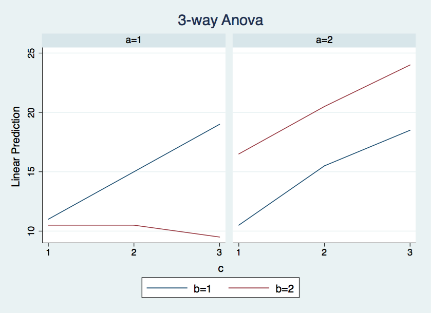
use https://stats.idre.ucla.edu/stat/data/3way, clear

anova y a##b##c

                           Number of obs =      24     R-squared     =  0.9689
                           Root MSE      =  1.1547     Adj R-squared =  0.9403

                  Source |  Partial SS    df       MS           F     Prob > F
              -----------+----------------------------------------------------
                   Model |  497.833333    11  45.2575758      33.94     0.0000
                         |
                       a |         150     1         150     112.50     0.0000
                       b |  .666666667     1  .666666667       0.50     0.4930
                     a#b |  160.166667     1  160.166667     120.13     0.0000
                       c |  127.583333     2  63.7916667      47.84     0.0000
                     a#c |       18.25     2       9.125       6.84     0.0104
                     b#c |  22.5833333     2  11.2916667       8.47     0.0051
                   a#b#c |  18.5833333     2  9.29166667       6.97     0.0098
                         |
                Residual |          16    12  1.33333333
              -----------+----------------------------------------------------
                   Total |  513.833333    23  22.3405797

* Compute cell means for plotting

quietly margins a#b#c

* Plot the cell means

marginsplot, recast(line) noci x(c) by(a) byopts(title(3-way Anova))


* Start by looking at the simple effects of the b#c interaction
at each level of a

contrast b#c@a

Contrasts of marginal linear predictions

Margins      : asbalanced

------------------------------------------------
             |         df           F        P>F
-------------+----------------------------------
       b#c@a |
          1  |          2       15.25     0.0005
          2  |          2        0.19     0.8314
      Joint  |          4        7.72     0.0026
             |
    Residual |         12
------------------------------------------------

* Follow up with the simple effects of b at each level of
c holding a at at 1

contrast b@c@1.a

Contrasts of marginal linear predictions

Margins      : asbalanced

------------------------------------------------
             |         df           F        P>F
-------------+----------------------------------
       b@c#a |
        1 1  |          1        0.19     0.6727
        2 1  |          1       15.19     0.0021
        3 1  |          1       67.69     0.0000
      Joint  |          3       27.69     0.0000
             |
    Residual |         12
------------------------------------------------

* Difference in differences

* b = 1 vs b = 2 when c = 2 and a = 1

contrast {b -1 1}@2.c@1.a

Contrasts of marginal linear predictions

Margins      : asbalanced

------------------------------------------------
             |         df           F        P>F
-------------+----------------------------------
       b@c#a |
    (1) 2 1  |          1       15.19     0.0021
             |
    Residual |         12
------------------------------------------------

--------------------------------------------------------------
             |   Contrast   Std. Err.     [95% Conf. Interval]
-------------+------------------------------------------------
       b@c#a |
    (1) 2 1  |       -4.5   1.154701     -7.015876   -1.984124
--------------------------------------------------------------

* since b has only two levels this is the same as

contrast b@2.c@1.a, effect

Contrasts of marginal linear predictions

Margins      : asbalanced

------------------------------------------------
             |         df           F        P>F
-------------+----------------------------------
       b@c#a |
        2 1  |          1       15.19     0.0021
             |
    Residual |         12
------------------------------------------------

------------------------------------------------------------------------------
             |   Contrast   Std. Err.      t    P>|t|     [95% Conf. Interval]
-------------+----------------------------------------------------------------
       b@c#a |
(2 vs base)  |
        2 1  |       -4.5   1.154701    -3.90   0.002    -7.015876   -1.984124
------------------------------------------------------------------------------

* Inspect L matrix

matrix list r(L)

r(L)[1,36]

                1b.     2.    1b.     2.  1b.a#  1b.a#  2o.a#   2.a#    1b.
                 a      a      b      b   1b.b   2o.b   1b.b    2.b      c
2.b@2.c@1.a      0      0     -1      1     -1      1      0      0      0


                 2.     3.  1b.a#  1b.a#  1b.a#  2o.a#   2.a#   2.a#  1b.b#
                 c      c   1b.c   2o.c   3o.c   1b.c    2.c    3.c   1b.c
2.b@2.c@1.a      0      0      0      0      0      0      0      0      0

                                                 1b.a#  1b.a#  1b.a#  1b.a#
              1b.b#  1b.b#  2o.b#   2.b#   2.b#  1b.b#  1b.b#  1b.b#  2o.b#
              2o.c   3o.c   1b.c    2.c    3.c   1b.c   2o.c   3o.c   1b.c
2.b@2.c@1.a     -1      0      0      1      0      0     -1      0      0

              1b.a#  1b.a#  2o.a#  2o.a#  2o.a#  2o.a#   2.a#   2.a#
              2o.b#  2o.b#  1b.b#  1b.b#  1b.b#  2o.b#   2.b#   2.b#
              2o.c   3o.c   1b.c   2o.c   3o.c   1b.c    2.c    3.c  _cons
2.b@2.c@1.a      1      0      0      0      0      0      0      0      0

* difference in levels of b between c = 2 and c = 3, when a = 1

contrast b#{c  0 -1 1}@1.a, effect

Contrasts of marginal linear predictions

Margins      : asbalanced

--------------------------------------------------
               |         df           F        P>F
---------------+----------------------------------
         b#c@a |
(joint) (1) 1  |          1        9.37     0.0099
               |
      Residual |         12
--------------------------------------------------

------------------------------------------------------------------------------
             |   Contrast   Std. Err.      t    P>|t|     [95% Conf. Interval]
-------------+----------------------------------------------------------------
       b#c@a |
(2 vs base)  |
      (1) 1  |         -5   1.632993    -3.06   0.010    -8.557986   -1.442014
------------------------------------------------------------------------------

* difference in levels of b between c = 2 and c = 3, when a = 2

contrast b#{c 0 -1 1}@2.a, effect

Contrasts of marginal linear predictions

Margins      : asbalanced

--------------------------------------------------
               |         df           F        P>F
---------------+----------------------------------
         b#c@a |
(joint) (1) 2  |          1        0.09     0.7647
               |
      Residual |         12
--------------------------------------------------

------------------------------------------------------------------------------
             |   Contrast   Std. Err.      t    P>|t|     [95% Conf. Interval]
-------------+----------------------------------------------------------------
       b#c@a |
(2 vs base)  |
      (1) 2  |         .5   1.632993     0.31   0.765    -3.057986    4.057986
------------------------------------------------------------------------------

* difference in differences in differences
* difference in levels of b between c = 2 and c = 3, when a = 1 vs a = 2

contrast b#{c 0 -1 1}#{a 1 -1}, effect

Contrasts of marginal linear predictions

Margins      : asbalanced

------------------------------------------------
             |         df           F        P>F
-------------+----------------------------------
       b#c#a |          1        5.67     0.0347
             |
    Residual |         12
------------------------------------------------

------------------------------------------------------------------------------
             |   Contrast   Std. Err.      t    P>|t|     [95% Conf. Interval]
-------------+----------------------------------------------------------------
       b#c#a |
(2 vs base)  |
    (1) (1)  |       -5.5   2.309401    -2.38   0.035    -10.53175   -.4682473
------------------------------------------------------------------------------

* Inspect L matrix again (nasty isn't it?)

matrix list r(L)

r(L)[1,36]

         1b.     2.    1b.     2.  1b.a#  1b.a#  2o.a#   2.a#    1b.     2.
          a      a      b      b   1b.b   2o.b   1b.b    2.b      c      c
2.b#
u1.c#
u1.a      0      0      0      0      0      0      0      0      0      0


          3.  1b.a#  1b.a#  1b.a#  2o.a#   2.a#   2.a#  1b.b#  1b.b#  1b.b#
          c   1b.c   2o.c   3o.c   1b.c    2.c    3.c   1b.c   2o.c   3o.c
2.b#
u1.c#
u1.a      0      0      0      0      0      0      0      0      0      0

                            1b.a#  1b.a#  1b.a#  1b.a#  1b.a#  1b.a#  2o.a#
       2o.b#   2.b#   2.b#  1b.b#  1b.b#  1b.b#  2o.b#  2o.b#  2o.b#  1b.b#
       1b.c    2.c    3.c   1b.c   2o.c   3o.c   1b.c   2o.c   3o.c   1b.c
2.b#
u1.c#
u1.a      0      0      0      0      1     -1      0     -1      1      0

       2o.a#  2o.a#  2o.a#   2.a#   2.a#
       1b.b#  1b.b#  2o.b#   2.b#   2.b#
       2o.c   3o.c   1b.c    2.c    3.c  _cons
2.b#
u1.c#
u1.a     -1      1      0      1     -1      0
* Start by looking at the simple effects of the b#c interaction
at each level of a
contrast b#c@a
Contrasts of marginal linear predictions
Margins : asbalanced
------------------------------------------------
| df F P>F
-------------+----------------------------------
b#c@a |
1 | 2 15.25 0.0005
2 | 2 0.19 0.8314
Joint | 4 7.72 0.0026
|
Residual | 12
------------------------------------------------
* Follow up with the simple effects of b at each level of
c holding a at at 1
contrast b@c@1.a
Contrasts of marginal linear predictions
Margins : asbalanced
------------------------------------------------
| df F P>F
-------------+----------------------------------
b@c#a |
1 1 | 1 0.19 0.6727
2 1 | 1 15.19 0.0021
3 1 | 1 67.69 0.0000
Joint | 3 27.69 0.0000
|
Residual | 12
------------------------------------------------
* Difference in differences
* b = 1 vs b = 2 when c = 2 and a = 1
contrast {b -1 1}@2.c@1.a
Contrasts of marginal linear predictions
Margins : asbalanced
------------------------------------------------
| df F P>F
-------------+----------------------------------
b@c#a |
(1) 2 1 | 1 15.19 0.0021
|
Residual | 12
------------------------------------------------
--------------------------------------------------------------
| Contrast Std. Err. [95% Conf. Interval]
-------------+------------------------------------------------
b@c#a |
(1) 2 1 | -4.5 1.154701 -7.015876 -1.984124
--------------------------------------------------------------
* since b has only two levels this is the same as
contrast b@2.c@1.a, effect
Contrasts of marginal linear predictions
Margins : asbalanced
------------------------------------------------
| df F P>F
-------------+----------------------------------
b@c#a |
2 1 | 1 15.19 0.0021
|
Residual | 12
------------------------------------------------
------------------------------------------------------------------------------
| Contrast Std. Err. t P>|t| [95% Conf. Interval]
-------------+----------------------------------------------------------------
b@c#a |
(2 vs base) |
2 1 | -4.5 1.154701 -3.90 0.002 -7.015876 -1.984124
------------------------------------------------------------------------------
* Inspect L matrix
matrix list r(L)
r(L)[1,36]
1b. 2. 1b. 2. 1b.a# 1b.a# 2o.a# 2.a# 1b.
a a b b 1b.b 2o.b 1b.b 2.b c
2.b@2.c@1.a 0 0 -1 1 -1 1 0 0 0
2. 3. 1b.a# 1b.a# 1b.a# 2o.a# 2.a# 2.a# 1b.b#
c c 1b.c 2o.c 3o.c 1b.c 2.c 3.c 1b.c
2.b@2.c@1.a 0 0 0 0 0 0 0 0 0
1b.a# 1b.a# 1b.a# 1b.a#
1b.b# 1b.b# 2o.b# 2.b# 2.b# 1b.b# 1b.b# 1b.b# 2o.b#
2o.c 3o.c 1b.c 2.c 3.c 1b.c 2o.c 3o.c 1b.c
2.b@2.c@1.a -1 0 0 1 0 0 -1 0 0
1b.a# 1b.a# 2o.a# 2o.a# 2o.a# 2o.a# 2.a# 2.a#
2o.b# 2o.b# 1b.b# 1b.b# 1b.b# 2o.b# 2.b# 2.b#
2o.c 3o.c 1b.c 2o.c 3o.c 1b.c 2.c 3.c _cons
2.b@2.c@1.a 1 0 0 0 0 0 0 0 0
* difference in levels of b between c = 2 and c = 3, when a = 1
contrast b#{c 0 -1 1}@1.a, effect
Contrasts of marginal linear predictions
Margins : asbalanced
--------------------------------------------------
| df F P>F
---------------+----------------------------------
b#c@a |
(joint) (1) 1 | 1 9.37 0.0099
|
Residual | 12
--------------------------------------------------
------------------------------------------------------------------------------
| Contrast Std. Err. t P>|t| [95% Conf. Interval]
-------------+----------------------------------------------------------------
b#c@a |
(2 vs base) |
(1) 1 | -5 1.632993 -3.06 0.010 -8.557986 -1.442014
------------------------------------------------------------------------------
* difference in levels of b between c = 2 and c = 3, when a = 2
contrast b#{c 0 -1 1}@2.a, effect
Contrasts of marginal linear predictions
Margins : asbalanced
--------------------------------------------------
| df F P>F
---------------+----------------------------------
b#c@a |
(joint) (1) 2 | 1 0.09 0.7647
|
Residual | 12
--------------------------------------------------
------------------------------------------------------------------------------
| Contrast Std. Err. t P>|t| [95% Conf. Interval]
-------------+----------------------------------------------------------------
b#c@a |
(2 vs base) |
(1) 2 | .5 1.632993 0.31 0.765 -3.057986 4.057986
------------------------------------------------------------------------------
* difference in differences in differences
* difference in levels of b between c = 2 and c = 3, when a = 1 vs a = 2
contrast b#{c 0 -1 1}#{a 1 -1}, effect
Contrasts of marginal linear predictions
Margins : asbalanced
------------------------------------------------
| df F P>F
-------------+----------------------------------
b#c#a | 1 5.67 0.0347
|
Residual | 12
------------------------------------------------
------------------------------------------------------------------------------
| Contrast Std. Err. t P>|t| [95% Conf. Interval]
-------------+----------------------------------------------------------------
b#c#a |
(2 vs base) |
(1) (1) | -5.5 2.309401 -2.38 0.035 -10.53175 -.4682473
------------------------------------------------------------------------------
* Inspect L matrix again (nasty isn't it?)
matrix list r(L)
r(L)[1,36]
1b. 2. 1b. 2. 1b.a# 1b.a# 2o.a# 2.a# 1b. 2.
a a b b 1b.b 2o.b 1b.b 2.b c c
2.b#
u1.c#
u1.a 0 0 0 0 0 0 0 0 0 0
3. 1b.a# 1b.a# 1b.a# 2o.a# 2.a# 2.a# 1b.b# 1b.b# 1b.b#
c 1b.c 2o.c 3o.c 1b.c 2.c 3.c 1b.c 2o.c 3o.c
2.b#
u1.c#
u1.a 0 0 0 0 0 0 0 0 0 0
1b.a# 1b.a# 1b.a# 1b.a# 1b.a# 1b.a# 2o.a#
2o.b# 2.b# 2.b# 1b.b# 1b.b# 1b.b# 2o.b# 2o.b# 2o.b# 1b.b#
1b.c 2.c 3.c 1b.c 2o.c 3o.c 1b.c 2o.c 3o.c 1b.c
2.b#
u1.c#
u1.a 0 0 0 0 1 -1 0 -1 1 0
2o.a# 2o.a# 2o.a# 2.a# 2.a#
1b.b# 1b.b# 2o.b# 2.b# 2.b#
2o.c 3o.c 1b.c 2.c 3.c _cons
2.b#
u1.c#
u1.a -1 1 0 1 -1 0
Model with categorical by continuous interaction
We will change to the hsbdemo dataset.
use https://stats.idre.ucla.edu/stat/data/hsbdemo, clear
anova math prog##c.read

                           Number of obs =     200     R-squared     =  0.5051
                           Root MSE      = 6.67488     Adj R-squared =  0.4924

                  Source |  Partial SS    df       MS           F     Prob > F
              -----------+----------------------------------------------------
                   Model |  8822.31169     5  1764.46234      39.60     0.0000
                         |
                    prog |  166.100182     2   83.050091       1.86     0.1578
                    read |  2926.41146     1  2926.41146      65.68     0.0000
               prog#read |  315.914185     2  157.957093       3.55     0.0307
                         |
                Residual |  8643.48331   194  44.5540377
              -----------+----------------------------------------------------
                   Total |   17465.795   199  87.7678141

* Used for plotting with two values, 25 & 75, for the continuous variable

quietly margins prog, at(read=(25 75))

* Plot it

marginsplot


* get slopes for each level of prog

margins prog, dydx(read)

Average marginal effects                          Number of obs   =        200

Expression   : Linear prediction, predict()
dy/dx w.r.t. : read

------------------------------------------------------------------------------
             |            Delta-method
             |      dy/dx   Std. Err.      z    P>|z|     [95% Conf. Interval]
-------------+----------------------------------------------------------------
read         |
        prog |
          1  |   .3180025   .1089668     2.92   0.004     .1044316    .5315735
          2  |    .629824   .0682596     9.23   0.000     .4960377    .7636103
          3  |   .4081276   .1070485     3.81   0.000     .1983165    .6179387
------------------------------------------------------------------------------

* Compare slopes using reference group contrast

margins r.prog, dydx(read)

Contrasts of average marginal effects

Expression   : Linear prediction, predict()
dy/dx w.r.t. : read

------------------------------------------------
             |         df        chi2     P>chi2
-------------+----------------------------------
read         |
        prog |
   (2 vs 1)  |          1        5.88     0.0153
   (3 vs 1)  |          1        0.35     0.5552
      Joint  |          2        7.09     0.0289
------------------------------------------------

--------------------------------------------------------------
             |   Contrast Delta-method
             |      dy/dx   Std. Err.     [95% Conf. Interval]
-------------+------------------------------------------------
read         |
        prog |
   (2 vs 1)  |   .3118215   .1285812       .059807     .563836
   (3 vs 1)  |    .090125   .1527519     -.2092631    .3895132
--------------------------------------------------------------

* Change reference group to prog3

margins rb2.prog, dydx(read)

Contrasts of average marginal effects

Expression   : Linear prediction, predict()
dy/dx w.r.t. : read

------------------------------------------------
             |         df        chi2     P>chi2
-------------+----------------------------------
read         |
        prog |
   (1 vs 2)  |          1        5.88     0.0153
   (3 vs 2)  |          1        3.05     0.0808
      Joint  |          2        7.09     0.0289
------------------------------------------------

--------------------------------------------------------------
             |   Contrast Delta-method
             |      dy/dx   Std. Err.     [95% Conf. Interval]
-------------+------------------------------------------------
read         |
        prog |
   (1 vs 2)  |  -.3118215   .1285812      -.563836    -.059807
   (3 vs 2)  |  -.2216965   .1269596     -.4705327    .0271398
--------------------------------------------------------------

* All pairwise slopes

margins prog, dydx(read) pwcompare(effects group)

Pairwise comparisons of average marginal effects

Expression   : Linear prediction, predict()
dy/dx w.r.t. : read

-------------------------------------------------
             |            Delta-method Unadjusted
             |     Margin   Std. Err.      Groups
-------------+-----------------------------------
read         |
        prog |
          1  |   .3180025   .1089668           A
          2  |    .629824   .0682596            B
          3  |   .4081276   .1070485           AB
-------------------------------------------------
Note: Margins sharing a letter in the group label
      are not significantly different at the 5%
      level.

------------------------------------------------------------------------------
             |   Contrast Delta-method    Unadjusted           Unadjusted
             |      dy/dx   Std. Err.      z    P>|z|     [95% Conf. Interval]
-------------+----------------------------------------------------------------
read         |
        prog |
     2 vs 1  |   .3118215   .1285812     2.43   0.015      .059807     .563836
     3 vs 1  |    .090125   .1527519     0.59   0.555    -.2092631    .3895132
     3 vs 2  |  -.2216965   .1269596    -1.75   0.081    -.4705327    .0271398
------------------------------------------------------------------------------

* User defined slope contrast

margins {prog -.5 1 -.5}, dydx(read)

Contrasts of average marginal effects

Expression   : Linear prediction, predict()
dy/dx w.r.t. : read

------------------------------------------------
             |         df        chi2     P>chi2
-------------+----------------------------------
read         |
        prog |          1        6.78     0.0092
------------------------------------------------

--------------------------------------------------------------
             |   Contrast Delta-method
             |      dy/dx   Std. Err.     [95% Conf. Interval]
-------------+------------------------------------------------
read         |
        prog |
        (1)  |    .266759   .1024336      .0659927    .4675252
--------------------------------------------------------------

* The same thing using contrast

contrast {prog -.5 1 -.5}#c.read

Contrasts of marginal linear predictions

Margins      : asbalanced

------------------------------------------------
             |         df           F        P>F
-------------+----------------------------------
 prog#c.read |          1        6.78     0.0099
             |
    Residual |        194
------------------------------------------------

--------------------------------------------------------------
             |   Contrast   Std. Err.     [95% Conf. Interval]
-------------+------------------------------------------------
 prog#c.read |
        (1)  |    .266759   .1024336      .0647324    .4687855
--------------------------------------------------------------
* get slopes for each level of prog
margins prog, dydx(read)
Average marginal effects Number of obs = 200
Expression : Linear prediction, predict()
dy/dx w.r.t. : read
------------------------------------------------------------------------------
| Delta-method
| dy/dx Std. Err. z P>|z| [95% Conf. Interval]
-------------+----------------------------------------------------------------
read |
prog |
1 | .3180025 .1089668 2.92 0.004 .1044316 .5315735
2 | .629824 .0682596 9.23 0.000 .4960377 .7636103
3 | .4081276 .1070485 3.81 0.000 .1983165 .6179387
------------------------------------------------------------------------------
* Compare slopes using reference group contrast
margins r.prog, dydx(read)
Contrasts of average marginal effects
Expression : Linear prediction, predict()
dy/dx w.r.t. : read
------------------------------------------------
| df chi2 P>chi2
-------------+----------------------------------
read |
prog |
(2 vs 1) | 1 5.88 0.0153
(3 vs 1) | 1 0.35 0.5552
Joint | 2 7.09 0.0289
------------------------------------------------
--------------------------------------------------------------
| Contrast Delta-method
| dy/dx Std. Err. [95% Conf. Interval]
-------------+------------------------------------------------
read |
prog |
(2 vs 1) | .3118215 .1285812 .059807 .563836
(3 vs 1) | .090125 .1527519 -.2092631 .3895132
--------------------------------------------------------------
* Change reference group to prog3
margins rb2.prog, dydx(read)
Contrasts of average marginal effects
Expression : Linear prediction, predict()
dy/dx w.r.t. : read
------------------------------------------------
| df chi2 P>chi2
-------------+----------------------------------
read |
prog |
(1 vs 2) | 1 5.88 0.0153
(3 vs 2) | 1 3.05 0.0808
Joint | 2 7.09 0.0289
------------------------------------------------
--------------------------------------------------------------
| Contrast Delta-method
| dy/dx Std. Err. [95% Conf. Interval]
-------------+------------------------------------------------
read |
prog |
(1 vs 2) | -.3118215 .1285812 -.563836 -.059807
(3 vs 2) | -.2216965 .1269596 -.4705327 .0271398
--------------------------------------------------------------
* All pairwise slopes
margins prog, dydx(read) pwcompare(effects group)
Pairwise comparisons of average marginal effects
Expression : Linear prediction, predict()
dy/dx w.r.t. : read
-------------------------------------------------
| Delta-method Unadjusted
| Margin Std. Err. Groups
-------------+-----------------------------------
read |
prog |
1 | .3180025 .1089668 A
2 | .629824 .0682596 B
3 | .4081276 .1070485 AB
-------------------------------------------------
Note: Margins sharing a letter in the group label
are not significantly different at the 5%
level.
------------------------------------------------------------------------------
| Contrast Delta-method Unadjusted Unadjusted
| dy/dx Std. Err. z P>|z| [95% Conf. Interval]
-------------+----------------------------------------------------------------
read |
prog |
2 vs 1 | .3118215 .1285812 2.43 0.015 .059807 .563836
3 vs 1 | .090125 .1527519 0.59 0.555 -.2092631 .3895132
3 vs 2 | -.2216965 .1269596 -1.75 0.081 -.4705327 .0271398
------------------------------------------------------------------------------
* User defined slope contrast
margins {prog -.5 1 -.5}, dydx(read)
Contrasts of average marginal effects
Expression : Linear prediction, predict()
dy/dx w.r.t. : read
------------------------------------------------
| df chi2 P>chi2
-------------+----------------------------------
read |
prog | 1 6.78 0.0092
------------------------------------------------
--------------------------------------------------------------
| Contrast Delta-method
| dy/dx Std. Err. [95% Conf. Interval]
-------------+------------------------------------------------
read |
prog |
(1) | .266759 .1024336 .0659927 .4675252
--------------------------------------------------------------
* The same thing using contrast
contrast {prog -.5 1 -.5}#c.read
Contrasts of marginal linear predictions
Margins : asbalanced
------------------------------------------------
| df F P>F
-------------+----------------------------------
prog#c.read | 1 6.78 0.0099
|
Residual | 194
------------------------------------------------
--------------------------------------------------------------
| Contrast Std. Err. [95% Conf. Interval]
-------------+------------------------------------------------
prog#c.read |
(1) | .266759 .1024336 .0647324 .4687855
--------------------------------------------------------------
For this last contrast we are not looking at differences in slopes but rather at differences in predicted values. In particular, we want to look at the differences among the three predicted values when read = 25 and again when read = 75.
* Differences in predicted values

margins r.prog, at(read=(25 75))

Contrasts of adjusted predictions

Expression   : Linear prediction, predict()

1._at        : read            =          25
2._at        : read            =          75

------------------------------------------------
             |         df        chi2     P>chi2
-------------+----------------------------------
    prog@_at |
 (2 vs 1) 1  |          1        1.92     0.1654
 (2 vs 1) 2  |          1       10.46     0.0012
 (3 vs 1) 1  |          1        1.34     0.2467
 (3 vs 1) 2  |          1        0.00     0.9773
      Joint  |          4       26.07     0.0000
------------------------------------------------

--------------------------------------------------------------
             |            Delta-method
             |   Contrast   Std. Err.     [95% Conf. Interval]
-------------+------------------------------------------------
    prog@_at |
 (2 vs 1) 1  |  -5.043076   3.635333      -12.1682    2.082046
 (2 vs 1) 2  |     10.548   3.261109      4.156342    16.93966
 (3 vs 1) 1  |  -4.382197   3.782612     -11.79598    3.031587
 (3 vs 1) 2  |   .1240545     4.3535     -8.408649    8.656758
--------------------------------------------------------------
That’s all for now.