This page presents examples of graphics programs written by Nicholas J. Cox
(Durham University). You can obtain these programs by typing, search command_name,
into the Stata command line and following the instructions (see
How can I use the search command to search for programs and get additional
help? for more information about using search). This page is not an exhaustive
list of all of the graphics commands written by Nick Cox but merely a collection of the
ones that we use most frequently. The command ssc install njc_stuff will download
two help files listing all programs written by Nick Cox, including his graph commands.This page contains only the commands and the plots themselves, there is no further explanation.
We envision that users will look through the plots and when they find one that appears
to do what they want, they will download the program and carefully read the help files.Most of these examples use the hsb2 dataset which can be downloaded from
within Stata using the following command:use https://stats.idre.ucla.edu/stat/data/hsb2, clearNote: Most of the graphs were produced using the scheme lean1. Whenever a different
scheme is used, it is given in the command.
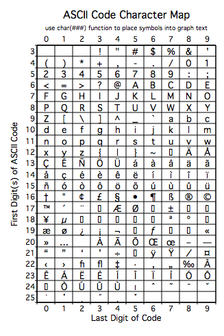
asciiplot– graph ASCII character set in current graph font
asciiplot
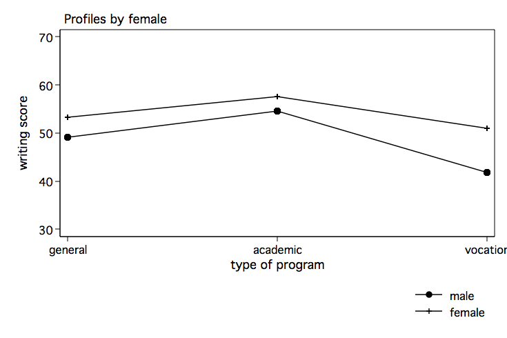
anovaplot– plot cell means following anova
anova write female prog female*prog anovaplot prog femaleanovaplot prog female, scatter(msym(i))
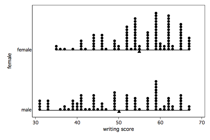
beamplot — horizontal dotplots using beams
beamplot writebeamplotplot write, over(female)
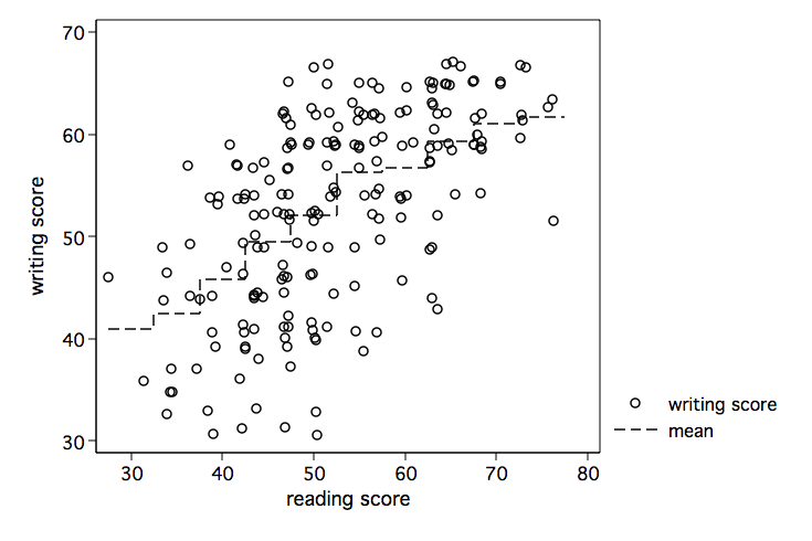
binsm — bin smoothing and summary on scatter plots
binsm write read, width(5) scatter(jitter(2))
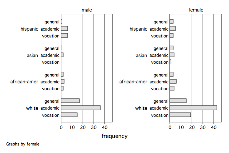
catplot — plots of categorical data
catplot prog racecatplot prog race, by(female)
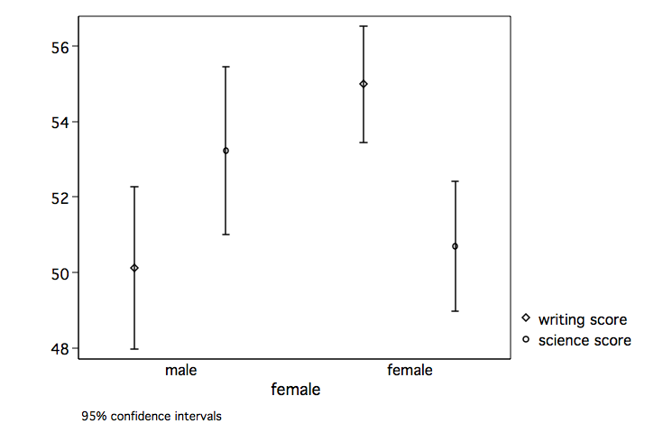
ciplot — plots of confidence intervals
ciplot write science, by(female)
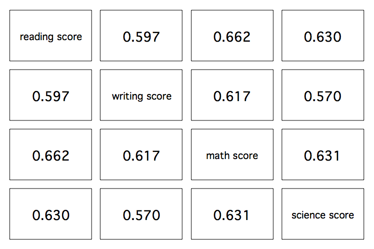
corrtable — correlation matrix as graphical table
corrtable read write math science
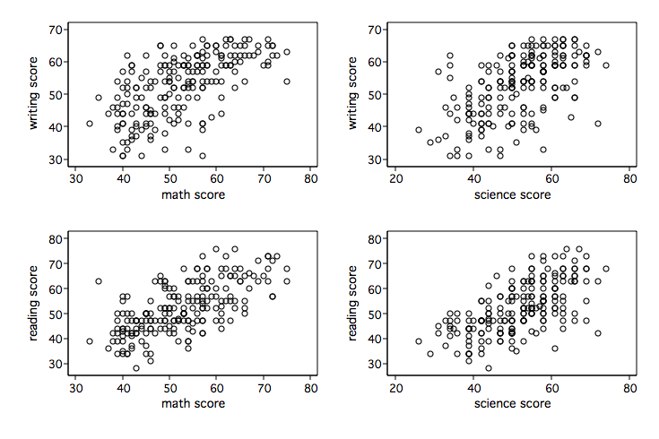
cpyxplot — twoway plots for each y vs each x
cpyxplot write \ read math science
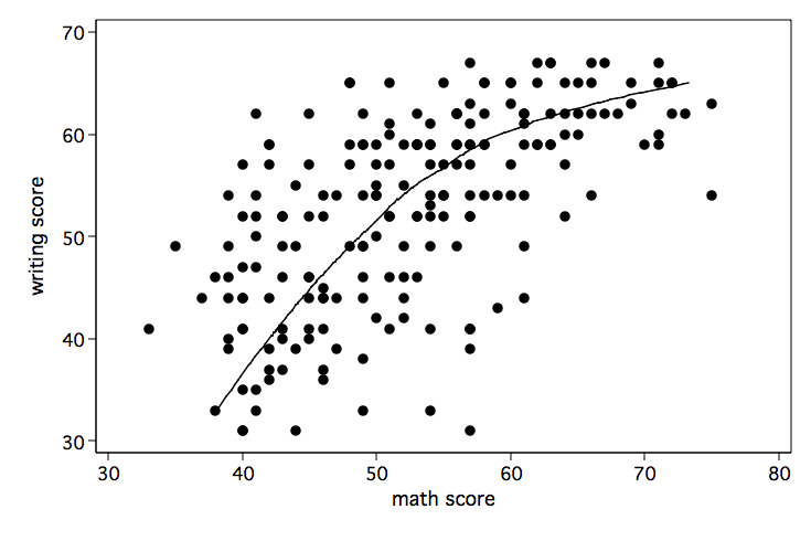
diagsm — diagonal smoothing
diagsm write math
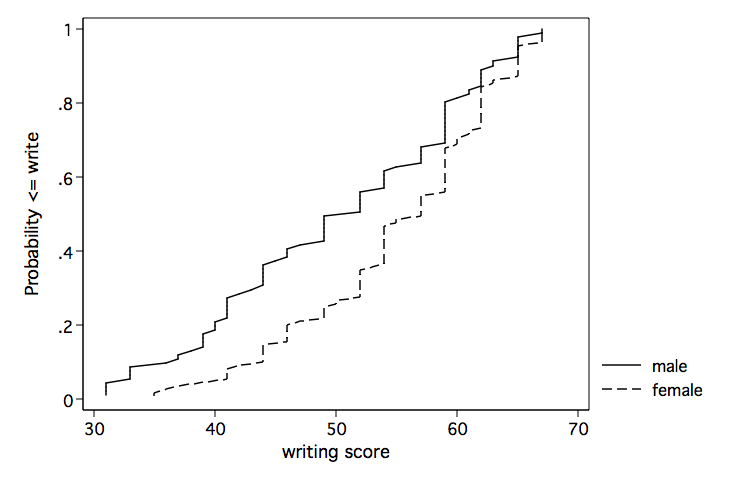
distplot — distribution function plots
distplot writedistplot write, over(female)
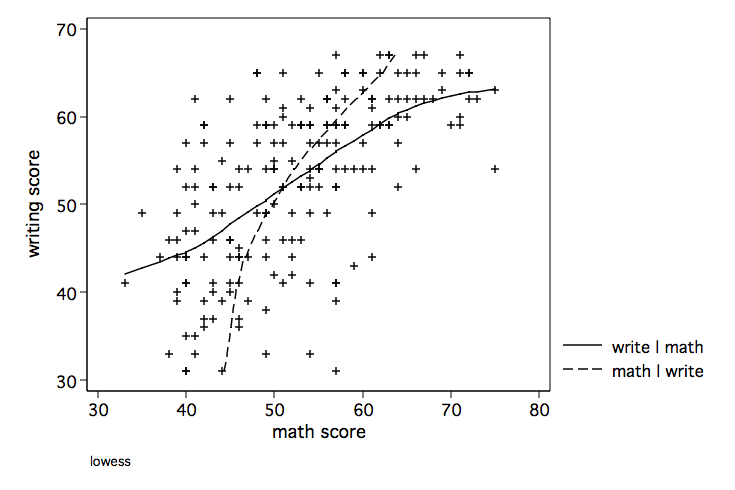
doublesm — double smoothing
doublesm write math
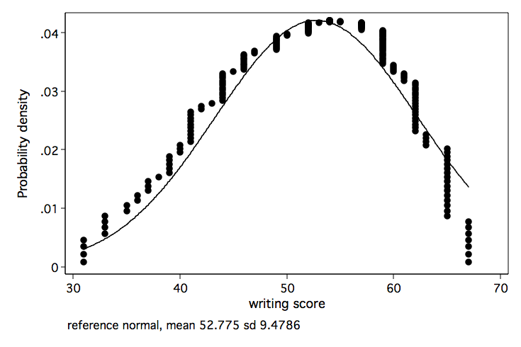
dpplot — density probability plots
dpplot write
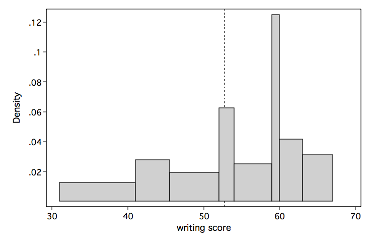
eqprhistogram — equal probability histograms
eqprhistogram write, mean
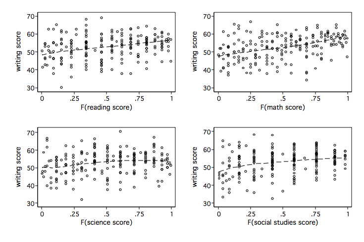
fractileplot — smoothing with distribution function predictors
fractileplot write read math science socst
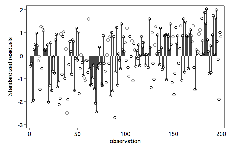
indexplot — index plots following estimation
regress write read indexplot, show(cooksd) hi(3)indexplot, show(rstandard) base(0)
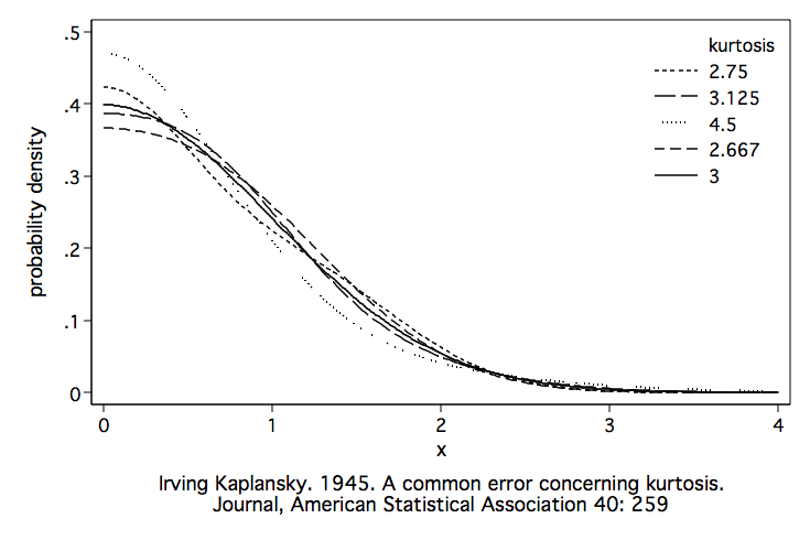
kaplansky — graph examples of distributions of varying kurtosis
kaplansky
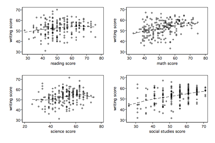
mlowess — lowess smoothing with multiple predictors
mlowess write read math science socst
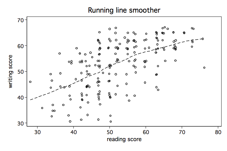
mrunning — running line smoother (multivariable version)
mrunning write read math
ovfplot
regress write read ovfplotregress write read female ovfplot, by(female)

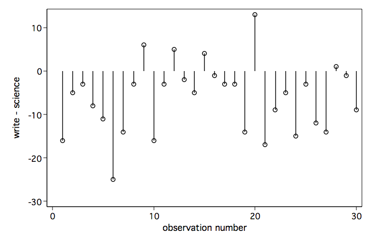
pairplot — plots of paired observations
pairplot write science in 1/30pairplot write science in 1/30, diff
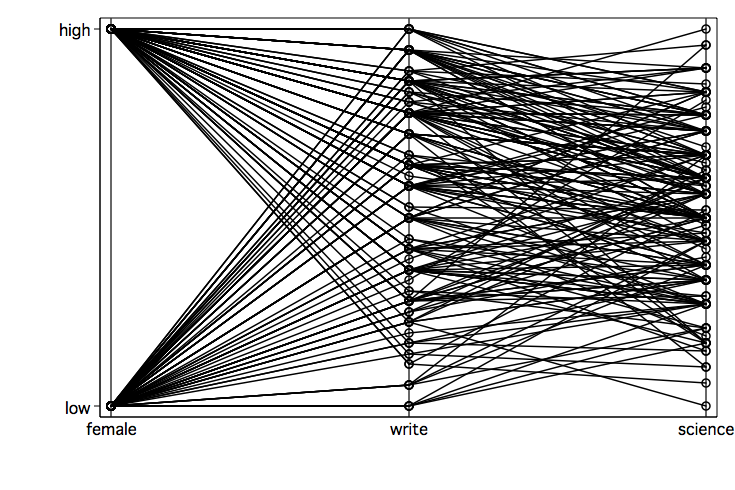
parplot — parallel coordinates plots
parplot female write science
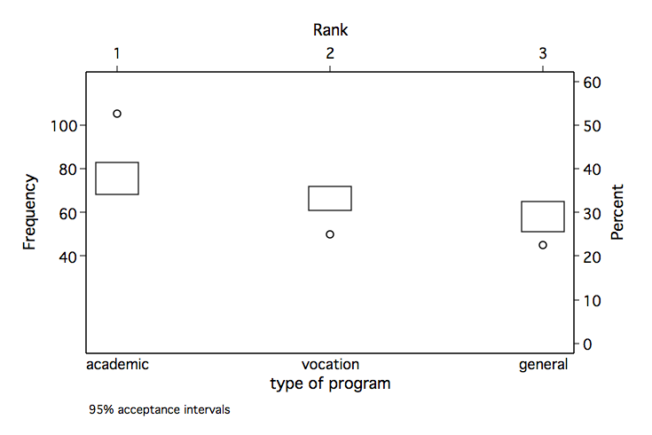
pdplot — Pareto dot plots
pdplot prog
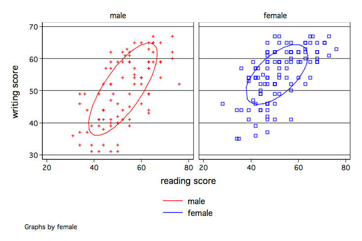
polarsm — polar smoothing
polarsm write read, over(female) by(female)
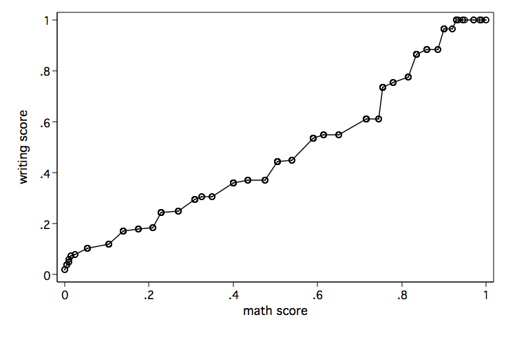
ppplot — P-P plots
ppplot connected write, by(female) ref(0)ppplot connected write math
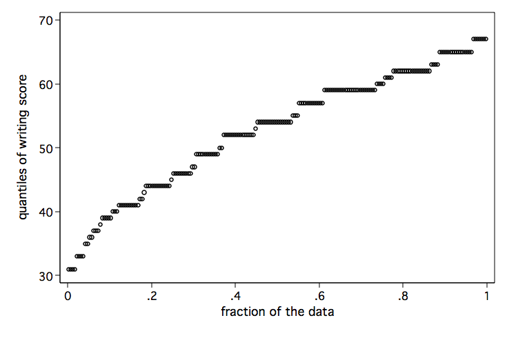
qplot — quantile plots
qplot write
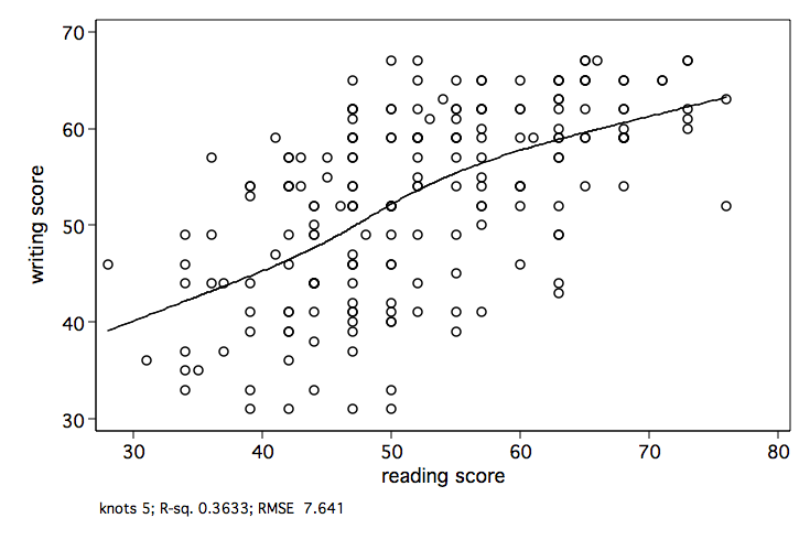
rcspline — restricted cubic spline smoothing
rcspline write read
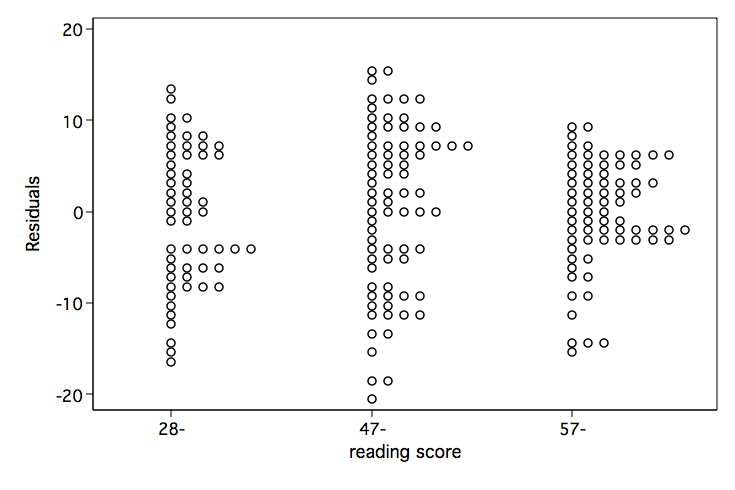
rdplot
regress write read
rdplot, g(3)
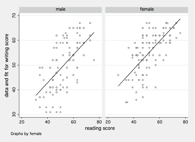
regplot
regress write read regplotgenerate write2 = write^2 regress math write write2 regplot
regress write read female regplot, by(female) scheme(s2mono)
rhetplot
regress write read
rhetplot, by(prog female)
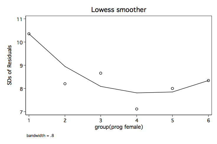
running — symmetric nearest neighbor smoothing
running write read, scatter(jitter(2))
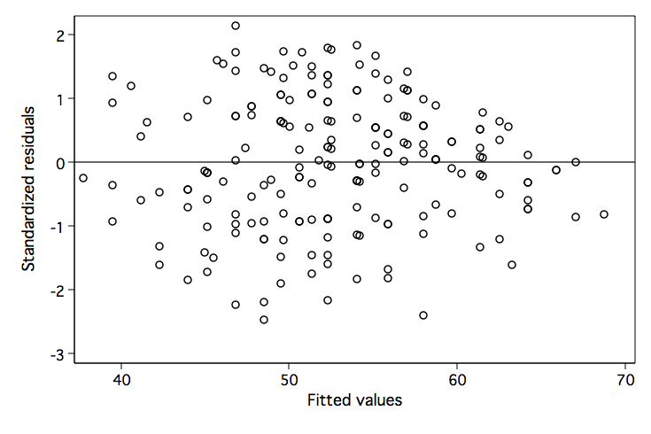
rvfplot2
regress write read female
rvfplot2, rstandard yline(0)
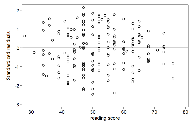
rvpplot2
regress write read female
rvpplot2 read, rstandard yline(0)
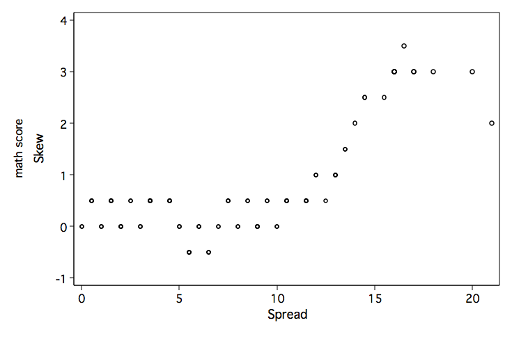
skewplot — skewness plots
skewplot math
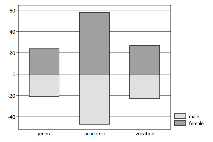
slideplot — sliding bar plots
slideplot bar female, pos(1) neg(0) by(prog)
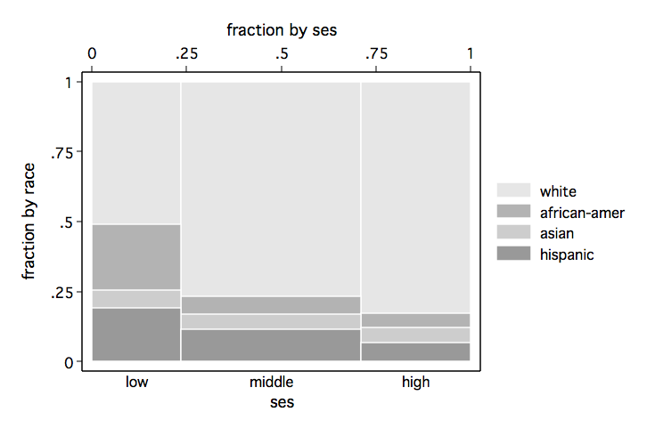
spineplot — spine plots for two-way categorical data
spineplot ses female, bar1(color(gs14)) bar2(color(gs10)) bar3(color(gs6))spineplot race ses
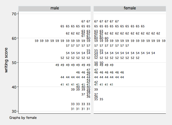
stemplot — stem-and-leaf plots
stemplot writestemplot write, d(2) by(female) back scheme(s2mono)
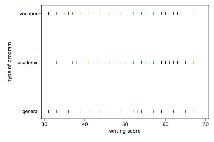
stripplot — strip plots
generate pipe = "|"
stripplot write, over(prog) mlabel(pipe) mlabpos(0) msymbol(i)
tableplot — graphical display in two-way table format
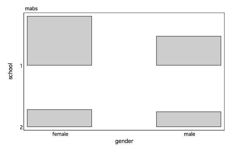
use https://stats.idre.ucla.edu/stat/stata/notes/lahigh, clear
egen mabs = mean(daysabs), by(school gender)
tableplot rbar mabs school gender
tabplot — two-way table shown as table of bars
use https://stats.idre.ucla.edu/stat/data/hsb2, clear
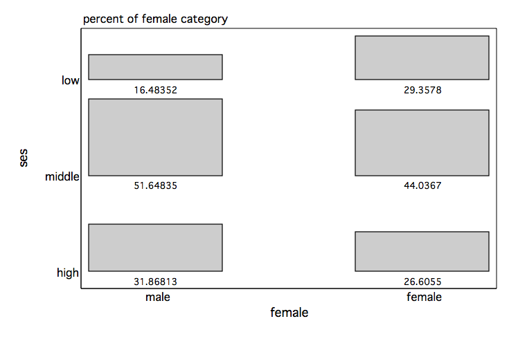
tabplot ses female, showval percent(female)