Let’s start off by down loading some data and running a binary mixed model with random intercepts and slopes.
use https://stats.idre.ucla.edu/stat/data/hsbdemo, clear

meqrlogit honors read i.female || cid: read, var covar(unstr)

Refining starting values:

Iteration 0:   log likelihood = -119.30049  (not concave)
Iteration 1:   log likelihood = -105.82055  (not concave)
Iteration 2:   log likelihood = -88.907174

Performing gradient-based optimization:

Iteration 0:   log likelihood = -88.907174  (not concave)
Iteration 1:   log likelihood = -84.544443  (not concave)
[output omitted]
Iteration 12:  log likelihood = -78.268094
Iteration 13:  log likelihood = -78.268094

Mixed-effects logistic regression               Number of obs      =       200
Group variable: cid                             Number of groups   =        20

                                                Obs per group: min =         7
                                                               avg =      10.0
                                                               max =        12

Integration points =   7                        Wald chi2(2)       =      8.29
Log likelihood = -78.268094                     Prob > chi2        =    0.0159

------------------------------------------------------------------------------
      honors |      Coef.   Std. Err.      z    P>|z|     [95% Conf. Interval]
-------------+----------------------------------------------------------------
        read |   .1084052   .0671505     1.61   0.106    -.0232074    .2400177
    1.female |   1.309964   .5183077     2.53   0.011        .2941    2.325829
       _cons |   -8.18226   3.894754    -2.10   0.036    -15.81584    -.548682
------------------------------------------------------------------------------

------------------------------------------------------------------------------
  Random-effects Parameters  |   Estimate   Std. Err.     [95% Conf. Interval]
-----------------------------+------------------------------------------------
cid: Unstructured            |
                   var(read) |   .0239163   .0244789      .0032171    .1777943
                  var(_cons) |   102.4491   96.65305      16.12367    650.9578
             cov(read,_cons) |   -1.55161   1.532405     -4.555068    1.451848
------------------------------------------------------------------------------
LR test vs. logistic regression:     chi2(3) =    14.35   Prob > chi2 = 0.0025

Note: LR test is conservative and provided only for reference.
Let’s try to use the margins command to get the predictive means (probabilities) for males and females holding the reading score at 50.
margins female, at(read=50) predict(mu)

prediction is a function of possibly stochastic quantities other than e(b)
It doesn’t work because the model has random effects in addition to the fixed effects. To get margins to work we need to include the predict(mu fixed) option.
margins female, at(read=50) predict(mu fixed)

Adjusted predictions                              Number of obs   =        200

Expression   : Predicted mean, fixed portion only, predict(mu fixed)
at           : read            =          50

------------------------------------------------------------------------------
             |            Delta-method
             |     Margin   Std. Err.      z    P>|z|     [95% Conf. Interval]
-------------+----------------------------------------------------------------
      female |
          0  |   .0594124   .0466851     1.27   0.203    -.0320887    .1509134
          1  |   .1896881   .1177394     1.61   0.107    -.0410769    .4204531
------------------------------------------------------------------------------
So, if margins won’t compute predictive margins with random effects we will have to compute them manually. We will begin with the easier task of computing predicted probabilities that include both the fixed and random effects. Of course, there is an option in predict that will do this. We will use predict, mu to check the results of our computation.
predict mu, mu // mu contains both fixed effects and random effects
Now we will replicate mu using the predicted random effects for both the intercept and the slope. These are the Best Linear Unbiased Predictors (BLUPs) also called empirical Bayes predictors.
predict re*, reffects

. describe re1 re2

              storage  display     value
variable name   type   format      label      variable label
--------------------------------------------------------------------------------------------------
re1             float  %9.0g                  random effects for cid: read
re2             float  %9.0g                  random effects for cid: _cons
We will use these BLUPs along with the coefficients from our model. The re2 values get added to the constant from the model and the re1 values are added to the coefficient for read. Since the variable rxb is in the log odds metric we need to exponentiate it to obtain predicted probabilities.
generate rxb = _b[1.female]*female + (_b[read]+re1)*read + (_b[_cons]+re2)

generate mu2 = exp(rxb)/(1+exp(rxb))

list mu mu2 in 1/20

     +---------------------+
     |       mu        mu2 |
     |---------------------|
  1. | .0068868   .0068868 |
  2. | .0018676   .0018676 |
  3. | .0041634   .0041634 |
  4. | .0030219   .0030219 |
  5. | .0041634   .0041634 |
     |---------------------|
  6. | .0244843   .0244843 |
  7. | .0011538   .0011538 |
  8. | .0239256   .0239256 |
  9. | .0152577   .0152577 |
 10. | .0018676   .0018676 |
     |---------------------|
 11. | .0068868   .0068868 |
 12. | .0039202   .0039202 |
 13. | .0142891   .0142891 |
 14. | .0088657   .0088658 |
 15. | .0075425   .0075425 |
     |---------------------|
 16. | .0088119   .0088119 |
 17. | .0024226   .0024226 |
 18. | .0232304   .0232304 |
 19. | .0017392   .0017392 |
 20. | .0017392   .0017392 |
     +---------------------+
The listing above shows that our manually computed mu2 is equal to the value mu generated by the predict command.
Let’s return to computing the predictive margins with random effect for males and females while holding reading at 50. In the code below rxb0 and rxb1 are the predictive margins in log odds for males and females respectively. To get the predictive margins in the probability metric we exponentiate the values to get p0 and p1. Again, the zero term is for males and the one term is for females.
generate rxb0 = _b[1.female]*0 + (_b[read]+re1)*50 + (_b[_cons]+re2)

generate rxb1 = _b[1.female]*1 + (_b[read]+re1)*50 + (_b[_cons]+re2)

generate p0 = exp(rxb0)/(1+exp(rxb0))

generate p1 = exp(rxb1)/(1+exp(rxb1))

summarize p0 p1

    Variable |       Obs        Mean    Std. Dev.       Min        Max
-------------+--------------------------------------------------------
          p0 |       200    .1755775    .2356444   .0125389    .829953
          p1 |       200    .3156575     .303865   .0449446   .9476115
These probabilities are rather different from the values we computed earlier using just the fixed effects. This highlights the fact that estimating predicated values while averaging over the fixed effects (e.g. predict) is not the same as estimating predicted values assuming the random effect is zero (e.g. margins) If we look at p0 and p1 within cid equal 1 we see that all the values for each variable are the same.
list p0 p1 if cid==1

     +---------------------+
     |       p0         p1 |
     |---------------------|
  1. | .0239256   .0832776 |
  2. | .0239256   .0832776 |
  3. | .0239256   .0832776 |
  4. | .0239256   .0832776 |
  5. | .0239256   .0832776 |
     |---------------------|
  6. | .0239256   .0832776 |
  7. | .0239256   .0832776 |
  8. | .0239256   .0832776 |
  9. | .0239256   .0832776 |
 10. | .0239256   .0832776 |
     |---------------------|
 11. | .0239256   .0832776 |
     +---------------------+
This means that the mean values computed by summarize above are influenced by the number of observations within each cid. That is, larger cids influence the mean more than smaller cids. To get around this we can use just one value from each cid. This will produce a more balanced predicted values. Here is a way to do this.
bysort cid: gen seq=_n

summarize p0 p1 if seq==1

    Variable |       Obs        Mean    Std. Dev.       Min        Max
-------------+--------------------------------------------------------
          p0 |        20    .1790172    .2416508   .0125389    .829953
          p1 |        20    .3212767    .3125198   .0449446   .9476115
Now we are ready to tackle a more complex model and set of predictive margins. We will add socst to our model as a covariate. But first, we will drop the variables we created above.
drop mu-p1

xtmelogit honors read female socst || cid: read, var covar(unstr)

Refining starting values:

Iteration 0:   log likelihood = -118.63766  (not concave)
Iteration 1:   log likelihood = -105.09158  (not concave)
Iteration 2:   log likelihood = -88.297585

Performing gradient-based optimization:

Iteration 0:   log likelihood = -88.297585  (not concave)
Iteration 1:   log likelihood = -83.769166  (not concave)
[output omitted]
Iteration 8:   log likelihood = -77.974955
Iteration 9:   log likelihood = -77.974949

Mixed-effects logistic regression               Number of obs      =       200
Group variable: cid                             Number of groups   =        20

                                                Obs per group: min =         7
                                                               avg =      10.0
                                                               max =        12

Integration points =   7                        Wald chi2(3)       =      9.12
Log likelihood = -77.974949                     Prob > chi2        =    0.0277

------------------------------------------------------------------------------
      honors |      Coef.   Std. Err.      z    P>|z|     [95% Conf. Interval]
-------------+----------------------------------------------------------------
        read |   .0980242   .0658639     1.49   0.137    -.0310668    .2271151
      female |   1.263858    .514295     2.46   0.014     .2558583    2.271858
       socst |   .0243635   .0317934     0.77   0.443    -.0379504    .0866774
       _cons |  -8.900997   3.842395    -2.32   0.021    -16.43195   -1.370041
------------------------------------------------------------------------------

------------------------------------------------------------------------------
  Random-effects Parameters  |   Estimate   Std. Err.     [95% Conf. Interval]
-----------------------------+------------------------------------------------
cid: Unstructured            |
                   var(read) |   .0209259   .0228458      .0024626    .1778206
                  var(_cons) |   89.13344   89.85624      12.35767     642.902
             cov(read,_cons) |  -1.353323   1.426992     -4.150175    1.443529
------------------------------------------------------------------------------
LR test vs. logistic regression:     chi2(3) =    12.38   Prob > chi2 = 0.0062

Note: LR test is conservative and provided only for reference.

predict re*, reffects
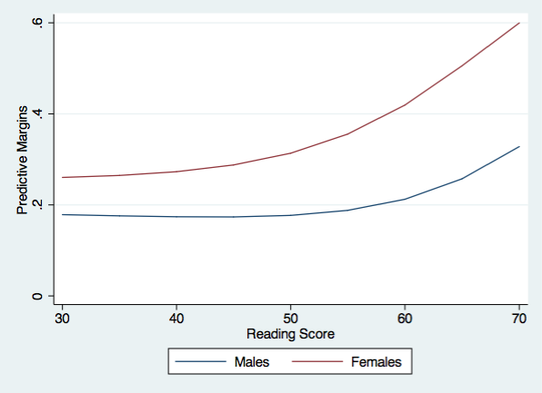
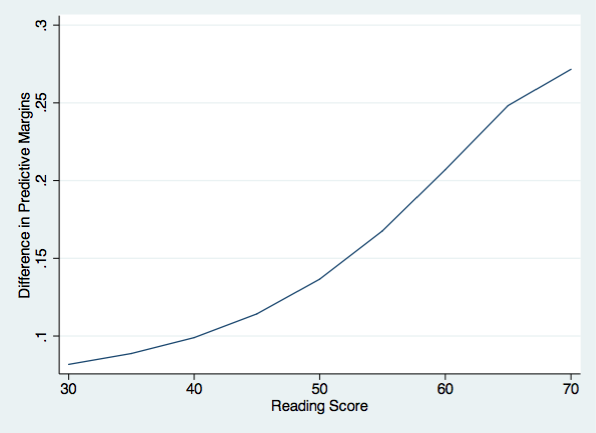
This time we want the predictive margins for males and females holding reading at values running from 30 to 70 in increments of five while leaving socst free to vary. We will do this with some temporary variables and three matrices: m predictive margins for males, f predictive margins for females and d the difference in predictive margins between males and females. Because of the local variables in the code below you will need to run the block of code all at one time, not one line at a time.
*** begin block ***

tempvar rxb0 rxb1 p0 p1
generate `rxb0' = .    // initialize temp var
generate `rxb1' = .    // initialize temp var
generate `p0' = .      // initialize temp var
generate `p1' = .      // initialize temp var
matrix m = J(9,1,0)    // initialize matrix for males
matrix f = J(9,1,0)    // initialize matrix for females
matrix d = J(9,1,0)    // initialize matrix for difference

local i = 1            // initialize local macro

forvalues j=30(5)70 {
quietly replace `rxb0' = _b[female]*0 + (_b[read]+re1)*`j' + _b[socst]*socst + _b[_cons]+re2
quietly replace `rxb1' = _b[female]*1 + (_b[read]+re1)*`j' + _b[socst]*socst + _b[_cons]+re2
quietly replace `p0' = exp(`rxb0')/(1+exp(`rxb0'))
quietly sum `p0'
matrix m[`i',1] = r(mean)
quietly replace `p1' = exp(`rxb1')/(1+exp(`rxb1'))
quietly sum `p1'
matrix f[`i',1] = r(mean)
matrix d[`i',1] = f[`i',1] - m[`i',1]
local i = `i' + 1      // increment local macro
}

*** end block ***
We can look at the predictive margins for males by listing matrix m.
matrix list m

m[9,1]
           c1
r1  .17859283
r2  .17596309
r3  .17393653
r4  .17354885
r5  .17695161
r6  .18797502
r7  .21236354
r8   .2572271
r9  .32805038
This first value above is the predictive margins for males with a reading score of 30 averaged across the observed values of socst. So, it does not matter that the number of observations differ within cid because the values of socst vary within cid.
Next, we will save the matrices as observations to our dataset.
matrix r = (303540455055606570)
svmat r
svmat m
svmat f
svmat d

list r1 m1 f1 d1 in 1/9

     +-------------------------------------+
     | r1         m1         f1         d1 |
     |-------------------------------------|
  1. | 30   .1785928   .2603539   .0817611 |
  2. | 35   .1759631   .2647262   .0887631 |
  3. | 40   .1739365   .2729119   .0989754 |
  4. | 45   .1735488   .2877812   .1142324 |
  5. | 50   .1769516   .3135495   .1365979 |
     |-------------------------------------|
  6. | 55    .187975   .3555776   .1676026 |
  7. | 60   .2123635   .4193873   .2070238 |
  8. | 65   .2572271   .5054632   .2482362 |
  9. | 70   .3280504   .5996285   .2715782 |
     +-------------------------------------+
Now we are ready to graph the predictive margins for males and females.
twoway (line m1 r1)(line f1 r1), ytitle(Predictive Margins) xtitle(Reading Score) ///
       legend(order(1 "Males" 2 "Females")) name(predictive, replace) ylabel(0(.2).6)

And finally, we can plot the difference between males and females in their predictive margins.
twoway (line d1 r1), ytitle(Difference in Predictive Margins) ///
       xtitle(Reading Score) name(difference, replace)

This general approach can be extended to more complex model with a concomitant increase in the complexity of our code.
