There are times when you want to do correspondence anlysis and the data have been collapsed into a summary with counts for each of the categories. For example, here is a table with the number of degrees given in 12 disciplines over eight different years.
discipline     1960       1965       1970       1971       1972       1973       1974       1975
    Agri        414        576        803        900        855        853        830        904
    Anth         69         82        217        240        260        324        381        385
     Bio       1245       1963       3360       3633       3580       3636       3473       3498
    Chem       1078       1444       2234       2204       2011       1849       1792       1762
   Earth        253        375        511        550        580        577        570        556
    Econ        341        538        826        791        863        907        833        867
     Eng        794       2073       3432       3495       3475       3338       3144       2959
    Math        291        685       1222       1236       1281       1222       1196       1149
     Oth        314        502       1079       1392       1500       1609       1531       1550
     Phy        530       1046       1655       1740       1635       1590        134       1293
   Psych        772        954       1888       2116       2262       2444       2587       2749
     Soc        162        239        504        583        638        599        645        680
We will begin by reading and describing the data.
use https://stats.idre.ucla.edu/stat/data/casummary, clear

describe

Contains data
  obs:            12
 vars:             9
 size:           480 (99.9% of memory free)
-------------------------------------------------------------------------------------------------------------
              storage  display     value
variable name   type   format      label      variable label
-------------------------------------------------------------------------------------------------------------
ndisc           long   %8.0g       ndisc
v60             float  %9.0g                  60 v
v65             float  %9.0g                  65 v
v70             float  %9.0g                  70 v
v71             float  %9.0g                  71 v
v72             float  %9.0g                  72 v
v73             float  %9.0g                  73 v
v74             float  %9.0g                  74 v
v75             float  %9.0g                  75 v
-------------------------------------------------------------------------------------------------------------
The problem is that we can’t run the ca when the data are in a wide format of summary data. The solution is to reshape the data into long form before running ca with frequency weights. Below you will see the reshape command and a partial listing of the reshaped data.
reshape long v, i(ndisc) j(y)

(note: j = 60 65 70 71 72 73 74 75)

Data                               wide   ->   long
-----------------------------------------------------------------------------
Number of obs.                       12   ->      96
Number of variables                   9   ->       3
j variable (8 values)                     ->   y
xij variables:
                        v60 v65 ... v75   ->   v
-----------------------------------------------------------------------------

clist in 1/15

        ndisc          y          v
  1.     Agri         60        414
  2.     Agri         65        576
  3.     Agri         70        803
  4.     Agri         71        900
  5.     Agri         72        855
  6.     Agri         73        853
  7.     Agri         74        830
  8.     Agri         75        904
  9.     Anth         60         69
 10.     Anth         65         82
 11.     Anth         70        217
 12.     Anth         71        240
 13.     Anth         72        260
 14.     Anth         73        324
 15.     Anth         74        381
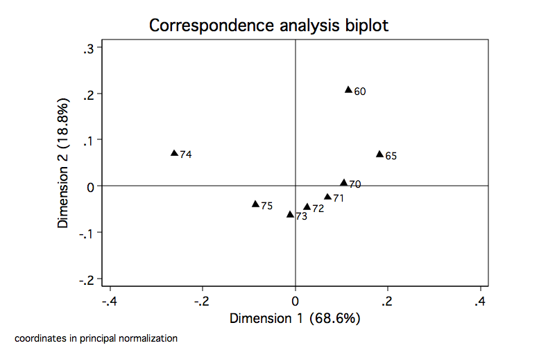
Now we are ready to run the correspondence analysis and plot the results.
ca ndisc y [fw=v], norm(principal)
Correspondence analysis Number of obs = 126707
Pearson chi2(77) = 2963.21
Prob > chi2 = 0.0000
Total inertia = 0.0234
12 active rows Number of dim. = 2
8 active columns Expl. inertia (%) = 87.38
| singular principal cumul
Dimension | value inertia chi2 percent percent
------------+------------------------------------------------------------
dim 1 | .1266166 .0160318 2031.34 68.55 68.55
dim 2 | .0663563 .0044032 557.91 18.83 87.38
dim 3 | .0496024 .0024604 311.75 10.52 97.90
dim 4 | .0149596 .0002238 28.36 0.96 98.86
dim 5 | .0128167 .0001643 20.81 0.70 99.56
dim 6 | .0079637 .0000634 8.04 0.27 99.83
dim 7 | .0062852 .0000395 5.01 0.17 100.00
------------+------------------------------------------------------------
total | .0233863 2963.21 100
Statistics for row and column categories in principal normalization
| overall | dimension_1 | dimension_2
Categories | mass quality %inert | coord sqcorr contrib | coord sqcorr contrib
-------------+---------------------------+---------------------------+---------------------------
ndisc | | |
Agri | 0.048 0.725 0.021 | 0.020 0.041 0.001 | 0.084 0.684 0.077
Anth | 0.015 0.925 0.055 | -0.273 0.893 0.072 | -0.052 0.032 0.009
Bio | 0.192 0.845 0.005 | -0.018 0.544 0.004 | 0.013 0.301 0.008
Chem | 0.113 0.983 0.129 | 0.100 0.378 0.071 | 0.127 0.605 0.415
Earth | 0.031 0.725 0.011 | 0.000 0.000 0.000 | 0.078 0.725 0.043
Econ | 0.047 0.462 0.008 | -0.003 0.003 0.000 | 0.043 0.460 0.020
Eng | 0.179 0.107 0.060 | 0.015 0.029 0.003 | -0.025 0.078 0.025
Math | 0.065 0.256 0.016 | -0.020 0.073 0.002 | -0.032 0.183 0.015
Oth | 0.075 0.949 0.102 | -0.147 0.684 0.101 | -0.092 0.265 0.143
Phy | 0.076 0.972 0.444 | 0.346 0.876 0.568 | -0.115 0.096 0.227
Psych | 0.124 0.838 0.122 | -0.139 0.835 0.149 | -0.009 0.004 0.002
Soc | 0.032 0.896 0.026 | -0.122 0.785 0.030 | -0.046 0.112 0.015
-------------+---------------------------+---------------------------+---------------------------
y | | |
60 | 0.049 0.763 0.155 | 0.114 0.178 0.040 | 0.207 0.585 0.480
65 | 0.083 0.900 0.148 | 0.182 0.790 0.170 | 0.068 0.110 0.086
70 | 0.140 0.821 0.080 | 0.105 0.818 0.096 | 0.006 0.002 0.001
71 | 0.149 0.867 0.040 | 0.069 0.769 0.045 | -0.025 0.098 0.021
72 | 0.149 0.883 0.020 | 0.025 0.201 0.006 | -0.046 0.682 0.073
73 | 0.150 0.806 0.033 | -0.011 0.026 0.001 | -0.063 0.780 0.135
74 | 0.135 0.968 0.436 | -0.261 0.904 0.575 | 0.069 0.064 0.148
75 | 0.145 0.635 0.088 | -0.086 0.518 0.067 | -0.041 0.117 0.055
-------------------------------------------------------------------------------------------------
cabiplot, origin
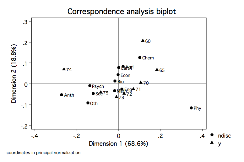 cabiplot, origin nocol
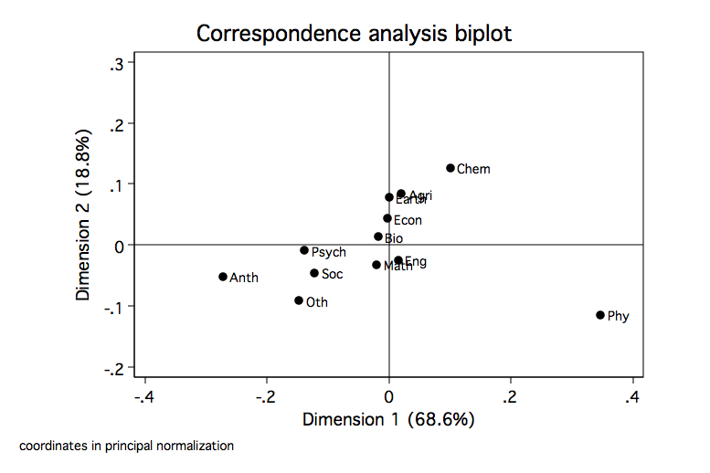 cabiplot, origin norow