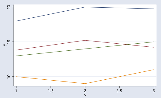
Profile analysis is performed using the manova command. The “trick” in doing profile analysis is to do transformations of the dependent variables, using the ytransform option, to allow for the testing of piecewise parallelism.
Example
This example profile analysis has four groups on three variables, labeled y1, y2 and y3. The plot of the profiles is shown below.

input id y1 y2 y3 grp
    1   19   20   18     1
    2   20   21   19     1
    3   19   22   22     1
    4   18   19   21     1
    5   16   18   20     1
    6   17   22   19     1
    7   20   19   20     1
    8   15   19   19     1
    9   12   14   12     2
   10   15   15   17     2
   11   15   17   15     2
   12   13   14   14     2
   13   14   16   13     2
   14   15   14   17     3
   15   13   14   15     3
   16   12   15   15     3
   17   12   13   13     3
   18    8    9   10     4
   19   10   10   12     4
   20   11   10   10     4
   21   11    7   12     4
end
tabstat y1 y2 y3, by(grp)
Summary statistics: mean
  by categories of: grp

     grp |        y1        y2        y3
---------+------------------------------
       1 |        18        20     19.75
       2 |      13.8      15.2      14.2
       3 |        13        14        15
       4 |        10         9        11
---------+------------------------------
   Total |  14.52381  15.61905  15.85714
----------------------------------------
/* preliminary one-way manova */
manova y1 y2 y3 = grp
                           Number of obs =      21

                           W = Wilks' lambda      L = Lawley-Hotelling trace
                           P = Pillai's trace     R = Roy's largest root

                  Source |  Statistic     df   F(df1,    df2) =   F   Prob>F
              -----------+--------------------------------------------------
                     grp | W   0.0479      3     9.0    36.7    10.12 0.0000 a
                         | P   1.1609            9.0    51.0     3.58 0.0016 a
                         | L  15.6417            9.0    41.0    23.75 0.0000 a
                         | R  15.3753            3.0    17.0    87.13 0.0000 u
                         |--------------------------------------------------
                Residual |                17
              -----------+--------------------------------------------------
                   Total |                20
              --------------------------------------------------------------
                           e = exact, a = approximate, u = upper bound on F
manovatest, showorder
Order of columns in the design matrix
      1: (grp==1)
      2: (grp==2)
      3: (grp==3)
      4: (grp==4)
      5: _cons
Please note that as of Stata 11, the _cons is the last element in the design matrix. In earlier versions of Stata, the _cons is the first element. This will make a difference in xm matrix below.
/* test of parallelism */
matrix c1 = (1,-1,0,1,-1)
manovatest grp, ytrans(c1)
 Transformations of the dependent variables

 (1)    y1 - y2
 (2)    y2 - y3

                           W = Wilks' lambda      L = Lawley-Hotelling trace
                           P = Pillai's trace     R = Roy's largest root

                  Source |  Statistic     df   F(df1,    df2) =   F   Prob>F
              -----------+--------------------------------------------------
                     grp | W   0.5633      3     6.0    32.0     1.77 0.1364 e
                         | P   0.4873            6.0    34.0     1.83 0.1234 a
                         | L   0.6853            6.0    30.0     1.71 0.1522 a
                         | R   0.5088            3.0    17.0     2.88 0.0662 u
                         |--------------------------------------------------
                Residual |                17
              --------------------------------------------------------------
                           e = exact, a = approximate, u = upper bound on F
/* test of levels (group differences) */
mat c2 = (1,1,1)
manovatest grp, ytrans(c2)
 Transformation of the dependent variables
 (1)    y1 + y2 + y3

                           W = Wilks' lambda      L = Lawley-Hotelling trace
                           P = Pillai's trace     R = Roy's largest root

                  Source |  Statistic     df   F(df1,    df2) =   F   Prob>F
              -----------+--------------------------------------------------
                     grp | W   0.0740      3     3.0    17.0    70.93 0.0000 e
                         | P   0.9260            3.0    17.0    70.93 0.0000 e
                         | L  12.5165            3.0    17.0    70.93 0.0000 e
                         | R  12.5165            3.0    17.0    70.93 0.0000 e
                         |--------------------------------------------------
                Residual |                17
              --------------------------------------------------------------
                           e = exact, a = approximate, u = upper bound on
/* test of flatness */
matrix xm = (.25,.25,.25,.25,1)
 /* the xm matrix used to select the contrast */
 /* Stata 11: matrix xm = (.25,.25,.25,.25,1) */
 /* Stata 10: matrix xm = (1,.25,.25,.25,.25) */
manovatest, test(xm) ytrans(c1)
 Transformations of the dependent variables
 (1)    y1 - y2
 (2)    y2 - y3

 Test constraint
 (1)    .25*1.grp + .25*2.grp + .25*3.grp + .25*4.grp + _cons = 0

                           W = Wilks' lambda      L = Lawley-Hotelling trace
                           P = Pillai's trace     R = Roy's largest root

                  Source |  Statistic     df   F(df1,    df2) =   F   Prob>F
              -----------+--------------------------------------------------
              manovatest | W   0.5637      1     2.0    16.0     6.19 0.0102 e
                         | P   0.4363            2.0    16.0     6.19 0.0102 e
                         | L   0.7739            2.0    16.0     6.19 0.0102 e
                         | R   0.7739            2.0    16.0     6.19 0.0102 e
                         |--------------------------------------------------
                Residual |                17
              --------------------------------------------------------------
                           e = exact, a = approximate, u = upper bound on F
In this example the test of parallelism was not significant, i.e., the profiles are parallel. The test of levels (groups differences) was significant, showing separation of the group profiles. The test of flatness was also significant indicating that the profiles were not flat.
