Stata does not have a built-in command to do tests of simple main effects, however ATS has developed a program that will perform them. You can you can the sme command by typing search sme (see How can I use the search command to search for programs and get additional help? for more information about using search).
Now, let’s read in an example dataset, crf24, adapted from Kirk (1968, 1st Edition).
use https://stats.idre.ucla.edu/stat/stata/faq/crf24, clear
These data are from a 2×4 factorial design. The variable y is the dependent variable. The variable a is an independent variable with two levels while b is an independent variable with four levels. Let’s look at a table of cell means and standard deviations.
table a b, contents(n y mean y sd y)

----------+---------------------------------------
          |                   b
        a |        1         2         3         4
----------+---------------------------------------
        1 |        4         4         4         4
          |     3.75         4         7         8
          |      1.5  .8164966  .8164966  .8164966
          |
        2 |        4         4         4         4
          |     1.75         3       5.5        10
          |       .5  .8164966  .5773503  .8164966
----------+---------------------------------------
Now let’s run the ANOVA.
anova y a b a*b

              Number of obs =      32     R-squared     =  0.9214
              Root MSE      = .877971     Adj R-squared =  0.8985

    Source |  Partial SS    df       MS           F     Prob > F
-----------+----------------------------------------------------
     Model |      217.00     7       31.00      40.22     0.0000
           |
         a |       3.125     1       3.125       4.05     0.0554
         b |      194.50     3  64.8333333      84.11     0.0000
       a*b |      19.375     3  6.45833333       8.38     0.0006
           |
  Residual |       18.50    24  .770833333
-----------+----------------------------------------------------
     Total |      235.50    31  7.59677419
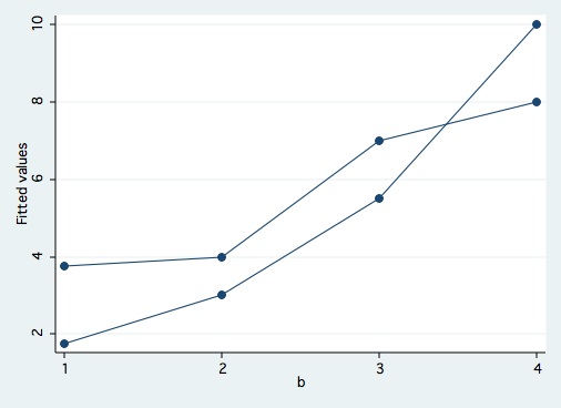
We see that in addition to a significant main effect for b there is a significant a*b interaction effect. Before we do any of the tests of simple main effects, let’s graph the cell means to get an idea of what the interaction looks like. The following sequence of commands will produce a graph of the cell means.
predict yhat
sort a b
graph twoway scatter yhat b, connect(L)
The interaction is clearly shown where the two lines cross over between levels b3 and b4. We will now do a test of simple main effects looking at differences in a at each level of b. In the sme command the first variable listed is the one being tested at each level of the second variable listed.
sme a b

Test of a at b(1): F(1/24)  = 10.378378
Test of a at b(2): F(1/24)  = 2.5945946
Test of a at b(3): F(1/24)  = 5.8378378
Test of a at b(4): F(1/24)  = 10.378378


Critical value of F for alpha = .05 using ...
-----------------------------------------------------------
Dunn's procedure              = 5.7165623
per family error rate         = 7.291317
simultaneous test procedure   = 12.090564
If we were to use the per family error rate then the differences in a at b1 and b4 would be statistically significant. And from the graph of the interaction we know that the differences are in opposite directions. Using the very conservative simultaneous test procedure none of the differences in a would be considered statistically significant. Using the criteria for Dunn’s procedure may result in finding too many significant effects.
Note:Statisticians do not universally approve of the use of tests of simple main effects. In particular, there are concerns over the conceptual error rate. Tests of simple main effects are one tool that can be useful in interpreting interactions. Caution should be exercised in interpreting the results produced by sme. In general, the results of tests of simple main effects should be considered suggestive and not definitive.

