Consider the following xtmelogit.
use https://stats.idre.ucla.edu/stat/data/hsbdemo, clear

xtmelogit honors i.female read || cid:

Refining starting values:

Iteration 0:   log likelihood = -82.156921
Iteration 1:   log likelihood = -80.132249
Iteration 2:   log likelihood = -79.765159

Performing gradient-based optimization:

Iteration 0:   log likelihood = -79.765159
Iteration 1:   log likelihood = -79.721813
Iteration 2:   log likelihood =  -79.72173
Iteration 3:   log likelihood =  -79.72173

Mixed-effects logistic regression               Number of obs      =       200
Group variable: cid                             Number of groups   =        20

                                                Obs per group: min =         7
                                                               avg =      10.0
                                                               max =        12

Integration points =   7                        Wald chi2(2)       =      6.39
Log likelihood =  -79.72173                     Prob > chi2        =    0.0410

------------------------------------------------------------------------------
      honors |      Coef.   Std. Err.      z    P>|z|     [95% Conf. Interval]
-------------+----------------------------------------------------------------
    1.female |   1.203685    .498816     2.41   0.016     .2260232    2.181346
        read |   .0426387   .0579243     0.74   0.462    -.0708908    .1561682
       _cons |  -4.827711   2.919208    -1.65   0.098    -10.54925    .8938321
------------------------------------------------------------------------------

------------------------------------------------------------------------------
  Random-effects Parameters  |   Estimate   Std. Err.     [95% Conf. Interval]
-----------------------------+------------------------------------------------
cid: Identity                |
                   sd(_cons) |   2.097709   .9227794      .8857332     4.96807
------------------------------------------------------------------------------
LR test vs. logistic regression: chibar2(01) =    11.44 Prob>=chibar2 = 0.0004
Say that we wanted to know the predicted probabilities for males and females at five different values of read, 30, 40, 50, 60 and 70. We might try using the margins command.
margins female, at(read=(30(10)70)) vsquish

default prediction is a function of possibly stochastic quantities other than e(b)
r(498);
That didn’t work because margins can’t compute predicted values for models that have both fixed and random components.
We can, however, get the predicted probabilities from just the fixed part of the model, like this.
margins female, at(read=(30(10)70)) predict(mu fixedonly) vsquish

Adjusted predictions                              Number of obs   =        200

Expression   : Predicted mean, fixed portion only, predict(mu fixedonly)
1._at        : read            =          30
2._at        : read            =          40
3._at        : read            =          50
4._at        : read            =          60
5._at        : read            =          70

------------------------------------------------------------------------------
             |            Delta-method
             |     Margin   Std. Err.      z    P>|z|     [95% Conf. Interval]
-------------+----------------------------------------------------------------
  _at#female |
        1 0  |    .027962   .0353643     0.79   0.429    -.0413509    .0972748
        1 1  |   .0874748   .1006056     0.87   0.385    -.1097085    .2846582
        2 0  |   .0422023   .0352079     1.20   0.231    -.0268039    .1112085
        2 1  |   .1280315   .0900429     1.42   0.155    -.0484494    .3045123
        3 0  |   .0632231   .0416911     1.52   0.129      -.01849    .1449363
        3 1  |   .1836082   .0928378     1.98   0.048     .0016494     .365567
        4 0  |   .0936902   .0807071     1.16   0.246    -.0644929    .2518733
        4 1  |   .2562211   .1691374     1.51   0.130     -.075282    .5877243
        5 0  |   .1366968   .1661537     0.82   0.411    -.1889584     .462352
        5 1  |   .3454012   .3085949     1.12   0.263    -.2594336    .9502361
------------------------------------------------------------------------------
For many purposes these probabilities from the fixed effects only will be all that we will need and these probabilities could be graphed using marginsplot. If we are specifically interested in the estimated of probabilities that include both fixed and random effects we can make use of the predict command.
First, we will estimate the predicted probabilities from the fixed and random parts of the model directly.
predict mu1, mu

tabstat  mu1, by(female)

Summary for variables: mu1
     by categories of: female

female |      mean
-------+----------
  male |  .1909927
female |  .3182445
-------+----------
 Total |  .2603449
------------------
The values produced by tabstat give us the predicted probabilities separately for males and females while read is held at its observed values. We can estimate these same values in two steps by estimating the linear predictor for the random and fixed effects separately.
predict re*, reffects  //  linear predictor for the random effects

predict xb, xb         // linear predictor for the fixed effects

gen mu2 = 1 /(1+exp(-1*(xb + re1)))  // compute probabilities using both fixed and random components

tabstat mu2, by(female)

Summary for variables: mu2
     by categories of: female

female |      mean
-------+----------
  male |  .1909927
female |  .3182445
-------+----------
 Total |  .2603449
------------------
As you can see the predicted probabilities computed this way are the same as when we predicted mu1 directly. The term (xb + re1) combines the fixed and random linear predictors while 1 /(1+exp(-1*(xb + re1))) converts the predictions to the probability metric.
We will now use the same approach to fix read at its mean value while letting female vary as observed.
sum read
replace read = r(mean)
predict xb3, xb
gen mu3 = 1 /(1+exp(-1*(xb3 + re1)))

tabstat mu3, by(female)

Summary for variables: mu3
     by categories of: female

female |      mean
-------+----------
  male |  .1588983
female |  .3037404
-------+----------
 Total |  .2378372
------------------
We can use this same method to compute predicted probabilities for each gender at the five values of read of interest by computing a separate xb for each combination of values. We can continue to use the the linear random predictor, re1, because the observations remain nested in the same cid. We will do the computations in a forvalues loop.
forvalues i=30(10)70 {
   quietly replace read = `i'
   quietly replace female = 0  // begin with the males
   predict xbm`i' , xb
   gen mum`i' = 1 /(1+exp(-1*(xbm`i' + re1)))
   quietly replace female = 1  // now for the females
   predict xbf`i' , xb
   gen muf`i' = 1 /(1+exp(-1*(xbf`i' + re1)))
}

sum mum* muf*

    Variable |       Obs        Mean    Std. Dev.       Min        Max
-------------+--------------------------------------------------------
       mum30 |       200    .0878644    .1277633   .0062536    .452949
       mum40 |       200    .1181626     .161502   .0095469   .5591283
       mum50 |       200    .1545762    .1959134   .0145493    .660161
       mum60 |       200    .1969638    .2284821   .0221143   .7484569
       mum70 |       200    .2450655    .2570279   .0334791   .8200648
-------------+--------------------------------------------------------
       muf30 |       200     .189036    .2229538   .0205396   .7339823
       muf40 |       200    .2361479    .2523496   .0311209   .8086573
       muf50 |       200    .2887174    .2762624   .0468924   .8661915
       muf60 |       200    .3463831    .2931488   .0700785   .9083859
       muf70 |       200    .4087083    .3014779   .1034842   .9382238
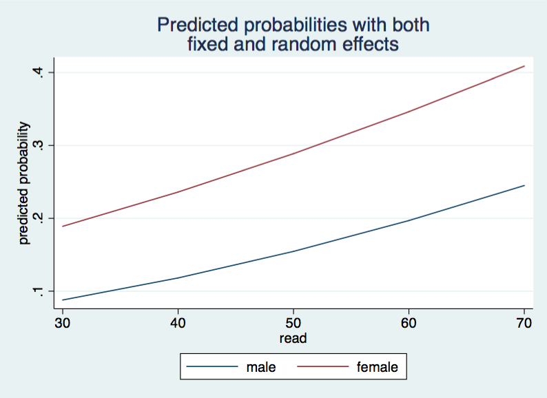
The variables that begin mum give the predicted values for the males for each of the five different values of read. The muf do the same thing for the females. We will plot these values by collapsing the data to a single observation and then reshaping the data long.
collapse (mean) mum* muf*
gen tid = 1
reshape long mum muf, i(tid) j(read)

twoway (line mum read)(line muf read), legend(order(1 "male" 2 "female")) ///
  ytitle(predicted probability) ///
  title("Predicted probabilities with both" "fixed and random effects") ///
  name(mu, replace)

With this approach you can replace the observed values with the mean values or any value that you wish. So, this approach worked okay for random intercepts, how would it work if we include a random coefficient (slope).
use https://stats.idre.ucla.edu/stat/data/hsbdemo, clear

xtmelogit honors i.female read || cid: female, cov(unstr)

Refining starting values:

Iteration 0:   log likelihood = -81.308446
Iteration 1:   log likelihood = -79.509044
Iteration 2:   log likelihood = -79.233888

Performing gradient-based optimization:

Iteration 0:   log likelihood = -79.233888
Iteration 1:   log likelihood = -79.203192
Iteration 2:   log likelihood =  -79.20305
Iteration 3:   log likelihood =  -79.20305

Mixed-effects logistic regression               Number of obs      =       200
Group variable: cid                             Number of groups   =        20

                                                Obs per group: min =         7
                                                               avg =      10.0
                                                               max =        12

Integration points =   7                        Wald chi2(2)       =      2.07
Log likelihood =  -79.20305                     Prob > chi2        =    0.3544

------------------------------------------------------------------------------
      honors |      Coef.   Std. Err.      z    P>|z|     [95% Conf. Interval]
-------------+----------------------------------------------------------------
    1.female |   1.107571   .9144827     1.21   0.226    -.6847819    2.899924
        read |   .0548958   .0614466     0.89   0.372    -.0655374    .1753289
       _cons |  -5.459728   3.237309    -1.69   0.092    -11.80474    .8852801
------------------------------------------------------------------------------

------------------------------------------------------------------------------
  Random-effects Parameters  |   Estimate   Std. Err.     [95% Conf. Interval]
-----------------------------+------------------------------------------------
cid: Unstructured            |
                  sd(female) |   1.270624    .877583      .3281837    4.919457
                   sd(_cons) |   2.104286   1.168272      .7088079    6.247133
          corr(female,_cons) |  -.1370656   1.016493     -.9741795    .9555909
------------------------------------------------------------------------------
LR test vs. logistic regression:     chi2(3) =    12.48   Prob > chi2 = 0.0059

Note: LR test is conservative and provided only for reference.

predict mu1, mu

tabstat mu1, by(female)

Summary for variables: mu1
     by categories of: female

female |      mean
-------+----------
  male |  .1884487
female |  .3188527
-------+----------
 Total |  .2595188
------------------
To reproduce the predicted probabilities that include both fixed and random effects, we need to obtain the linear predictor of the random effects as follows:
predict re*, reffects // obtain the random effects

des re*

              storage  display     value
variable name   type   format      label      variable label
--------------------------------------------------------------------------------------------
read            byte   %9.0g                  reading score
re1             float  %9.0g                  random effects for cid: female
re2             float  %9.0g                  random effects for cid: _cons
As you can see, re1 is the linear predictor for the random coefficient while re2 linear the linear predictor for the random intercept.
Now we need to compute the interaction of female with re1, obtain the linear predictor for the fixed effect and compute the probability.
gen fre1=female*re1

predict xb2, xb

gen mu2 = 1 /(1+exp(-1*(xb2 + fre1 + re2)))

tabstat mu2, by(female)

Summary for variables: mu2
     by categories of: female

female |      mean
-------+----------
  male |  .1884487
female |  .3188527
-------+----------
 Total |  .2595188
------------------
Once again mu1 and mu2 are the same.
Next, with this knowledge, we are going to compute the predicted probabilities for read for the values 30, 40 50 60 and 70 for both males and females, just like we did in the first section. This time we need to compute fre1 for both males and female. For male the value of female*re1 is zero. While for female the value of female*re1 is equal to re1.
forvalues i=30(10)70 {
  quietly replace read = `i'
  quietly replace female = 0
  quietly replace fre1 = 0  // this value is 0 for males
  predict xbm`i' , xb
  gen mum`i' = 1 /(1+exp(-1*(xbm`i' +fre1 + re2)))
  quietly replace female = 1
  quietly replace fre1 = re1  // this value is re1 for females
  predict xbf`i' , xb
  gen muf`i' = 1 /(1+exp(-1*(xbf`i' + fre1 + re2)))
}

sum mum* muf*

    Variable |       Obs        Mean    Std. Dev.       Min        Max
-------------+--------------------------------------------------------
       mum30 |       200     .067521    .1073255   .0062084   .4335063
       mum40 |       200    .1006205    .1453719    .010701   .5698889
       mum50 |       200    .1441323    .1850342   .0183843   .6964301
       mum60 |       200    .1988144    .2226292    .031409   .7988807
       mum70 |       200    .2647876    .2545738   .0531617   .8730579
-------------+--------------------------------------------------------
       muf30 |       200    .1651364    .2082666   .0140494   .5906218
       muf40 |       200    .2210162     .252848   .0240784   .7141231
       muf50 |       200    .2841479    .2869894    .040969   .8122126
       muf60 |       200    .3544923    .3071029   .0688718   .8821978
       muf70 |       200     .432452    .3113492   .1135287   .9283999
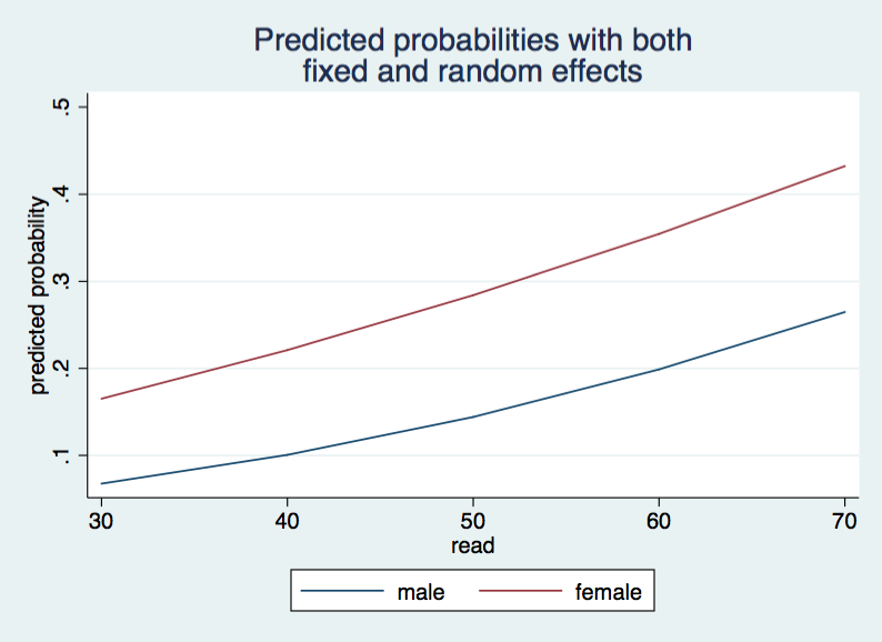
As before we will collapse the data then reshape them prior to plotting.
collapse (mean) mum* muf*
gen tid = 1
reshape long mum muf, i(tid) j(read)

twoway (line mum read)(line muf read), legend(order(1 "male" 2 "female")) ///
  ytitle(predicted probability) ///
  title("Predicted probabilities with both" "fixed and random effects") ///
  name(mu2, replace)

The two graphs that we generated for this page look very similar but inspection of the tables for the predicted probabilities show that adding the random coefficient to the model changes the predicted probabilities. Let’s check the two models using a likelihood-ratio test.
use https://stats.idre.ucla.edu/stat/data/hsbdemo, clear

quietly xtmelogit honors i.female read || cid: female, cov(unstr)
estimates store m1
quietly xtmelogit honors i.female read || cid:
estimates store m2

lrtest m1 m2

Likelihood-ratio test                                 LR chi2(2)  =      1.04
(Assumption: m1 nested in m2)                         Prob > chi2 =    0.5953

Note: The reported degrees of freedom assumes the null hypothesis is not on the boundary
      of the parameter space.  If this is not true, then the reported test is
      conservative.
So, in this instance, the model with the random coefficient is not significantly better than the model with just the random intercept.
Acknowledgements: Thanks to Jurjen Iedema of the Netherlands Institute for Social Research / SCP for suggesting this approach.
