
First off, let’s start with what a significant continuous by continuous interaction means.
It means that the slope of one continuous variable on the response variable changes as the
values on a second continuous change.
Multiple regression models often contain interaction terms. This FAQ page
covers the situation in which there is a moderator
variable which influences the regression of the dependent
variable on an independent/predictor variable. In other words, a regression
model that has a significant two-way interaction of continuous variables.
There are several approaches that one might use to
explain an interaction of two continuous variables.
The approach that we will demonstrate is to compute simple slopes, i.e., the
slopes of the dependent variable on the independent variable when the moderator variable is held constant at
different combinations of values from very low to very high.
We will consider a regression model which includes a continuous by
continuous interaction of a predictor variable with a moderator variable. In the formula, Y is the response variable, X the predictor
(independent) variable with Z being the moderator variable. The term XZ is the
interaction of the predictor with the moderator.
Y = b0 + b1X + b2Z + b3XZ
We will illustrate the simple slopes process using the hsbdemo dataset that has a
statistically significant continuous by continuous interaction. As shown in the code below
that read is the response variable,
math is the predictor and socst is the moderator variable.
use https://stats.idre.ucla.edu/stat/data/hsbdemo, clear

/* some descriptive statistics */

sum read math socst

    Variable |       Obs        Mean    Std. Dev.       Min        Max
-------------+--------------------------------------------------------
        read |       200       52.23    10.25294         28         76
        math |       200      52.645    9.368448         33         75
       socst |       200      52.405    10.73579         26         71

corr read math socst

(obs=200)

             |     read     math    socst
-------------+---------------------------
        read |   1.0000
        math |   0.6623   1.0000
       socst |   0.6215   0.5445   1.0000
Now, let’s run our regression model.
regress read c.math##c.socst

      Source |       SS       df       MS              Number of obs =     200
-------------+------------------------------           F(  3,   196) =   78.61
       Model |  11424.7622     3  3808.25406           Prob > F      =  0.0000
    Residual |  9494.65783   196  48.4421318           R-squared     =  0.5461
-------------+------------------------------           Adj R-squared =  0.5392
       Total |    20919.42   199  105.122714           Root MSE      =    6.96

------------------------------------------------------------------------------
        read |      Coef.   Std. Err.      t    P>|t|     [95% Conf. Interval]
-------------+----------------------------------------------------------------
        math |  -.1105123   .2916338    -0.38   0.705    -.6856552    .4646307
       socst |  -.2200442   .2717539    -0.81   0.419    -.7559812    .3158928
             |
      c.math#|
     c.socst |   .0112807   .0052294     2.16   0.032     .0009677    .0215938
             |
       _cons |   37.84271   14.54521     2.60   0.010     9.157506    66.52792
------------------------------------------------------------------------------
Please note that the interaction, c.math#c.socst, is statistically significant with
a p-value of 0.032.
Next, we compute the slope for read on math while holding
the value of the moderator variable, socst, constant at values running from 30 to 75.
To do this we will use the margins command, introduced in Stata 11, with a range of
values for socst using the at option.
margins, dydx(math) at(socst=(30(5)75)) vsquish

Average marginal effects                          Number of obs   =        200
Model VCE    : OLS

Expression   : Linear prediction, predict()
dy/dx w.r.t. : math
1._at        : socst           =          30
2._at        : socst           =          35
3._at        : socst           =          40
4._at        : socst           =          45
5._at        : socst           =          50
6._at        : socst           =          55
7._at        : socst           =          60
8._at        : socst           =          65
9._at        : socst           =          70
10._at       : socst           =          75

------------------------------------------------------------------------------
             |            Delta-method
             |      dy/dx   Std. Err.      z    P>|z|     [95% Conf. Interval]
-------------+----------------------------------------------------------------
math         |
         _at |
          1  |   .2279094   .1424924     1.60   0.110    -.0513706    .5071894
          2  |    .284313   .1195771     2.38   0.017     .0499463    .5186797
          3  |   .3407166   .0982883     3.47   0.001     .1480752     .533358
          4  |   .3971202   .0799363     4.97   0.000      .240448    .5537924
          5  |   .4535238   .0669803     6.77   0.000      .322245    .5848027
          6  |   .5099274   .0628508     8.11   0.000     .3867422    .6331127
          7  |   .5663311   .0691477     8.19   0.000     .4308041     .701858
          8  |   .6227347   .0835458     7.45   0.000     .4589878    .7864815
          9  |   .6791383   .1026924     6.61   0.000     .4778649    .8804117
         10  |   .7355419   .1244141     5.91   0.000     .4916947    .9793891
------------------------------------------------------------------------------
The values in the margins command gives the amount of change in read with
a one unit change in math while holding socst constant at different values,
i.e., the values are simple slopes. It appears that the simple slopes for math are
significant for all values of socst except when socst equals 30.
Next, we would like to plot these simple slopes for each of the values of socst. we
will use the the margins command again but place place math inside the at
option. We only need two values of math for each value of socst to define the
regression line for graphing purposes
margins, at(math=(30 75) socst=(30(5)70)) vsquish

Adjusted predictions                              Number of obs   =        200
Model VCE    : OLS

Expression   : Linear prediction, predict()
1._at        : math            =          30
               socst           =          30
2._at        : math            =          30
               socst           =          35
3._at        : math            =          30
               socst           =          40
4._at        : math            =          30
               socst           =          45
5._at        : math            =          30
               socst           =          50
6._at        : math            =          30
               socst           =          55
7._at        : math            =          30
               socst           =          60
8._at        : math            =          30
               socst           =          65
9._at        : math            =          30
               socst           =          70
10._at       : math            =          75
               socst           =          30
11._at       : math            =          75
               socst           =          35
12._at       : math            =          75
               socst           =          40
13._at       : math            =          75
               socst           =          45
14._at       : math            =          75
               socst           =          50
15._at       : math            =          75
               socst           =          55
16._at       : math            =          75
               socst           =          60
17._at       : math            =          75
               socst           =          65
18._at       : math            =          75
               socst           =          70

------------------------------------------------------------------------------
             |            Delta-method
             |     Margin   Std. Err.      z    P>|z|     [95% Conf. Interval]
-------------+----------------------------------------------------------------
         _at |
          1  |   38.07867   2.768479    13.75   0.000     32.65255    43.50479
          2  |   38.67056   2.271317    17.03   0.000     34.21886    43.12226
          3  |   39.26245   1.844077    21.29   0.000     35.64812    42.87677
          4  |   39.85433   1.545864    25.78   0.000     36.82449    42.88417
          5  |   40.44622   1.458119    27.74   0.000     37.58836    43.30408
          6  |   41.03811   1.615506    25.40   0.000     37.87177    44.20444
          7  |      41.63   1.959833    21.24   0.000     37.78879     45.4712
          8  |   42.22188   2.412336    17.50   0.000     37.49379    46.94997
          9  |   42.81377   2.923204    14.65   0.000     37.08439    48.54315
         10  |   48.33459   4.100129    11.79   0.000     40.29849     56.3707
         11  |   51.46464   3.459941    14.87   0.000     44.68328      58.246
         12  |   54.59469   2.841761    19.21   0.000     49.02494    60.16444
         13  |   57.72474    2.26369    25.50   0.000     53.28799    62.16149
         14  |   60.85479   1.765578    34.47   0.000     57.39432    64.31526
         15  |   63.98484   1.433357    44.64   0.000     61.17551    66.79417
         16  |   67.11489   1.391418    48.23   0.000     64.38776    69.84202
         17  |   70.24494   1.661882    42.27   0.000     66.98771    73.50217
         18  |   73.37499   2.128836    34.47   0.000     69.20255    77.54743
------------------------------------------------------------------------------
Now, we can plot the simple slopes using the marginsplot command introduced in Stata 12.
marginsplot, noci x(math) recast(line) xlabel(30(5)75)
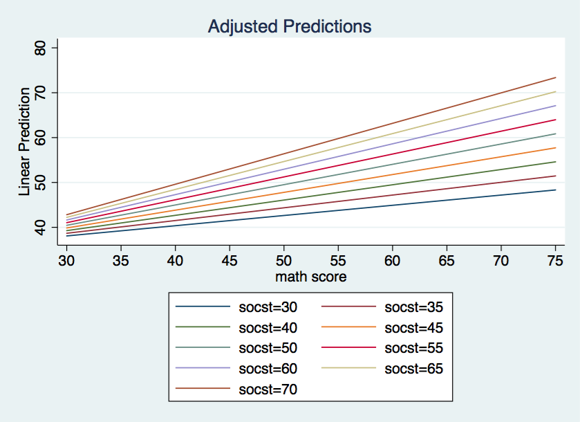
This graph is fine but it would look even better if we added in a scatterplot of the observed data points.
We can do this in marginsplot using the addplot option.
marginsplot, noci x(math) recast(line) ///
       addplot(scatter read math, msym(oh) jitter(3)) xlabel(35(10)75)
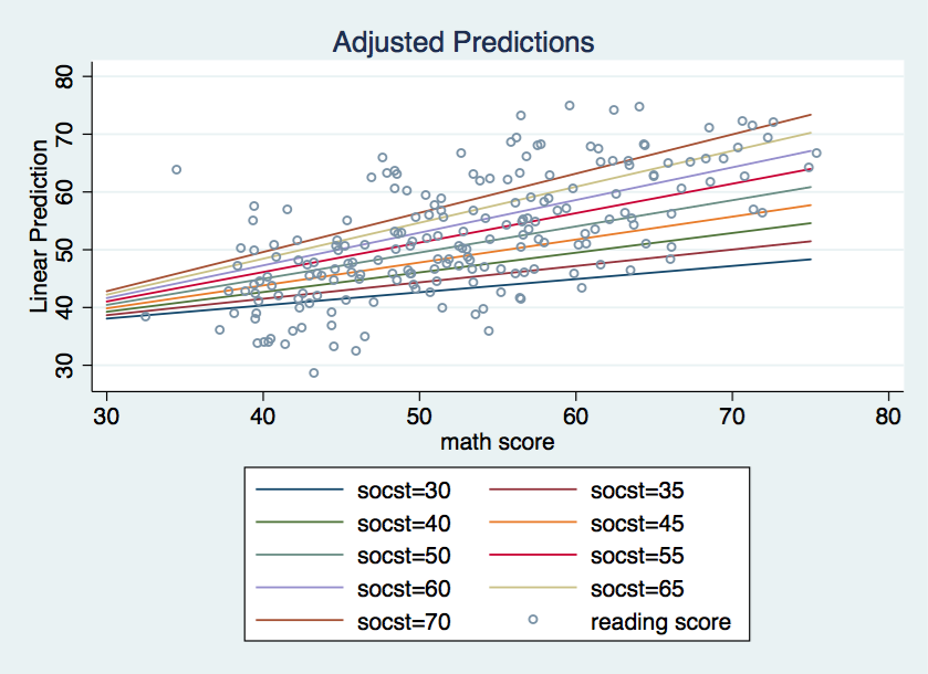
This is one way of interpreting a continuous by continuous interaction using Stata 12 and newer.