Stata 12 introduces many new commands. In this FAQ we will look at the contrast command and shown how it can be used to explore interactons. This page will show some of the ways you can explore interations. But, of course we cannot cover every possible method that is included in the contrast command.
Note: The techniques shown on this page are considered to ben post-hoc analyses. As such, they require the researcher to compute adjusted p-values for the various contrasts and tests. We will not show how to adjust the p-values in this presentation so that we can focus on the methods involving the contrast command.
We will begin by loading the data and running an anova model. The data are taken from Roger Kirk’s (1995) text on experimental design.
use https://stats.idre.ucla.edu/stat/stata/examples/kirk/crf33, clear

anova y a##b


                           Number of obs =      45     R-squared     =  0.5690
                           Root MSE      = 7.90569     Adj R-squared =  0.4732

                  Source |  Partial SS    df       MS           F     Prob > F
              -----------+----------------------------------------------------
                   Model |        2970     8      371.25       5.94     0.0001
                         |
                       a |         190     2          95       1.52     0.2324
                       b |  1543.33333     2  771.666667      12.35     0.0001
                     a#b |  1236.66667     4  309.166667       4.95     0.0028
                         |
                Residual |        2250    36        62.5
              -----------+----------------------------------------------------
                   Total |        5220    44  118.636364
Many researchers run their analyses using regression methods. We want to demonstrate that the contrast command works just as well with regression as it does with anova so we will rerun the model using the regress command.
regress y i.a##i.b

                  Source |       SS           df       MS      Number of obs   =        45
            -------------+----------------------------------   F(8, 36)        =      5.94
                   Model |        2970         8      371.25   Prob > F        =    0.0001
                Residual |        2250        36        62.5   R-squared       =    0.5690
            -------------+----------------------------------   Adj R-squared   =    0.4732
                   Total |        5220        44  118.636364   Root MSE        =    7.9057

            ------------------------------------------------------------------------------
                       y |      Coef.   Std. Err.      t    P>|t|     [95% Conf. Interval]
            -------------+----------------------------------------------------------------
                       a |
                      2  |         -3          5    -0.60   0.552    -13.14047     7.14047
                      3  |        -13          5    -2.60   0.013    -23.14047    -2.85953
                         |
                       b |
                      2  |          2          5     0.40   0.692     -8.14047    12.14047
                      3  |          5          5     1.00   0.324     -5.14047    15.14047
                         |
                     a#b |
                    2 2  |         -1   7.071068    -0.14   0.888    -15.34079    13.34079
                    2 3  |          1   7.071068     0.14   0.888    -13.34079    15.34079
                    3 2  |         18   7.071068     2.55   0.015      3.65921    32.34079
                    3 3  |         27   7.071068     3.82   0.001     12.65921    41.34079
                         |
                   _cons |         33   3.535534     9.33   0.000      25.8296     40.1704
            ------------------------------------------------------------------------------
We explicitly identified a and b as categorical (factor) variables. However, regress assumes that the interaction of two variables involves factor variables so we could chave written the commandas follows: regress y a##b. Since we ran the model as a regression we need to check to see if the interactions is significant using the contrast command.
contrast a#b

Contrasts of marginal linear predictions

Margins      : asbalanced

------------------------------------------------
             |         df           F        P>F
-------------+----------------------------------
         a#b |          4        4.95     0.0028
             |
    Residual |         36
------------------------------------------------
Not only is it significant, the F-ratio is identical to the anova results. This is because anova and regression are really two variants of the same linear model.
Next, we will use the margins command to get the nine cell means.
margins a#b

Adjusted predictions                              Number of obs   =         45

Expression   : Linear prediction, predict()

------------------------------------------------------------------------------
             |            Delta-method
             |     Margin   Std. Err.      z    P>|z|     [95% Conf. Interval]
-------------+----------------------------------------------------------------
         a#b |
        1 1  |         33   3.535534     9.33   0.000     26.07048    39.92952
        1 2  |         35   3.535534     9.90   0.000     28.07048    41.92952
        1 3  |         38   3.535534    10.75   0.000     31.07048    44.92952
        2 1  |         30   3.535534     8.49   0.000     23.07048    36.92952
        2 2  |         31   3.535534     8.77   0.000     24.07048    37.92952
        2 3  |         36   3.535534    10.18   0.000     29.07048    42.92952
        3 1  |         20   3.535534     5.66   0.000     13.07048    26.92952
        3 2  |         40   3.535534    11.31   0.000     33.07048    46.92952
        3 3  |         52   3.535534    14.71   0.000     45.07048    58.92952
------------------------------------------------------------------------------
Now, Let’s plot these means using the marginsplot command that was also introduced in Stata 12.
marginsplot, noci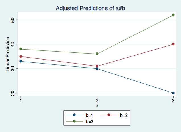
Okay, now we’re ready to explore this interacton.
Simple Contrasts
We will begin with some simple contrasts, that is, one degree of freedom contrasts for a variable run at each level of another variable. In this example, we will contrasts versus a reference category for variable a (level 1) at each level of variable b. The r. prefix indicates that we want to use reference category coding. The @ character indicates that we want this for each level of variable b. The effects option difplays addition output including t-tests and p-values.
contrast r.a@b, effects

Contrasts of marginal linear predictions

Margins      : asbalanced

------------------------------------------------
             |         df           F        P>F
-------------+----------------------------------
         a@b |
 (2 vs 1) 1  |          1        0.36     0.5523
 (2 vs 1) 2  |          1        0.64     0.4290
 (2 vs 1) 3  |          1        0.16     0.6915
 (3 vs 1) 1  |          1        6.76     0.0134
 (3 vs 1) 2  |          1        1.00     0.3240
 (3 vs 1) 3  |          1        7.84     0.0082
      Joint  |          6        3.80     0.0049
             |
    Residual |         36
------------------------------------------------

------------------------------------------------------------------------------
             |   Contrast   Std. Err.      t    P>|t|     [95% Conf. Interval]
-------------+----------------------------------------------------------------
         a@b |
 (2 vs 1) 1  |         -3          5    -0.60   0.552    -13.14047     7.14047
 (2 vs 1) 2  |         -4          5    -0.80   0.429    -14.14047     6.14047
 (2 vs 1) 3  |         -2          5    -0.40   0.692    -12.14047     8.14047
 (3 vs 1) 1  |        -13          5    -2.60   0.013    -23.14047    -2.85953
 (3 vs 1) 2  |          5          5     1.00   0.324     -5.14047    15.14047
 (3 vs 1) 3  |         14          5     2.80   0.008      3.85953    24.14047
------------------------------------------------------------------------------
Looking through these results, we see that the only significant contrasts are 3 vs 1 at b1 and at b3.
Simple Effects
A step up from simple contrasts are simple effects. We want to know whether the effect of a is significant at each level of variable b or not. Again we use the @ character to indicate that the tests are to be done at each level of b.
contrast a@b

Contrasts of marginal linear predictions

Margins      : asbalanced

------------------------------------------------
             |         df           F        P>F
-------------+----------------------------------
         a@b |
          1  |          2        3.71     0.0344
          2  |          2        1.63     0.2107
          3  |          2        6.08     0.0053
      Joint  |          6        3.80     0.0049
             |
    Residual |         36
------------------------------------------------
Each of these simple effects tests uses two degrees of freedom. The results indicate that the effects of a at b1 and a at b3 are significant. By refering to the earlier simple contrasts, it is clear that these significant simple effects are due to the 3 vs 1 at b1 and at b3.
Partial Interaction
Let’s look at the plot of the interaction again.
Partial interactions can allow us to ask questions about parts of out interaction. For instance, are the blue and red lines parallel? How about the read and the green lines? We will use the .a prefix to indicate adjacent levels of variable b.
contrast a#a.b

Contrasts of marginal linear predictions

Margins      : asbalanced

-----------------------------------------------------
                  |         df           F        P>F
------------------+----------------------------------
              a#b |
(joint) (1 vs 2)  |          2        4.57     0.0170
(joint) (2 vs 3)  |          2        0.89     0.4182
           Joint  |          4        4.95     0.0028
                  |
         Residual |         36
-----------------------------------------------------
We see that the blue versus red lines of b (1 vs 2) show a signifivant effect meaning that the lines are not parallel. While the red versys green (2 vs 3) effect is not significant, indicating parallelism. But what about the blue versus green (1 vs 3) lines. For this, we will run another one degree of freedom contrast. This time we will create a user defined contrast comparing b1 versus b3.
contrast a#{b 1 0 -1}

Contrasts of marginal linear predictions

Margins      : asbalanced

------------------------------------------------
             |         df           F        P>F
-------------+----------------------------------
         a#b |          2        9.37     0.0005
             |
    Residual |         36
------------------------------------------------
This contrast is also significant so the lines for b1 and b3 are not parallel.
Treatment Contrast Interactions
There are times when we will want to look at interactions of arbitrary contrasts. Each of these treatment contrasts are one degree of freedom. We will begin with reference group (r. prefix) contrasts for both a and b.
contrast r.a#r.b, effects

Contrasts of marginal linear predictions

Margins      : asbalanced

------------------------------------------------------
                   |         df           F        P>F
-------------------+----------------------------------
               a#b |
(2 vs 1) (2 vs 1)  |          1        0.02     0.8883
(2 vs 1) (3 vs 1)  |          1        0.02     0.8883
(3 vs 1) (2 vs 1)  |          1        6.48     0.0153
(3 vs 1) (3 vs 1)  |          1       14.58     0.0005
            Joint  |          4        4.95     0.0028
                   |
          Residual |         36
------------------------------------------------------

------------------------------------------------------------------------------------
                   |   Contrast   Std. Err.      t    P>|t|     [95% Conf. Interval]
-------------------+----------------------------------------------------------------
               a#b |
(2 vs 1) (2 vs 1)  |         -1   7.071068    -0.14   0.888    -15.34079    13.34079
(2 vs 1) (3 vs 1)  |          1   7.071068     0.14   0.888    -13.34079    15.34079
(3 vs 1) (2 vs 1)  |         18   7.071068     2.55   0.015      3.65921    32.34079
(3 vs 1) (3 vs 1)  |         27   7.071068     3.82   0.001     12.65921    41.34079
------------------------------------------------------------------------------------
The output indicates that the 3vs1 by 2vs1 interaction is significant along with the 3vs1 by 3vs1 interaction.
For this example, we used the same r. prefix (reference group) for both variables but we didn’t need to do this. We could have use r. for variable a and the a. prefix (adjacent group) for variable b. Here’s what that would look like.
contrast r.a#a.b, effects

Contrasts of marginal linear predictions

Margins      : asbalanced

------------------------------------------------------
                   |         df           F        P>F
-------------------+----------------------------------
               a#b |
(2 vs 1) (1 vs 2)  |          1        0.02     0.8883
(2 vs 1) (2 vs 3)  |          1        0.08     0.7789
(3 vs 1) (1 vs 2)  |          1        6.48     0.0153
(3 vs 1) (2 vs 3)  |          1        1.62     0.2113
            Joint  |          4        4.95     0.0028
                   |
          Residual |         36
------------------------------------------------------

------------------------------------------------------------------------------------
                   |   Contrast   Std. Err.      t    P>|t|     [95% Conf. Interval]
-------------------+----------------------------------------------------------------
               a#b |
(2 vs 1) (1 vs 2)  |          1   7.071068     0.14   0.888    -13.34079    15.34079
(2 vs 1) (2 vs 3)  |         -2   7.071068    -0.28   0.779    -16.34079    12.34079
(3 vs 1) (1 vs 2)  |        -18   7.071068    -2.55   0.015    -32.34079    -3.65921
(3 vs 1) (2 vs 3)  |         -9   7.071068    -1.27   0.211    -23.34079     5.34079
------------------------------------------------------------------------------------
Trend Interactions
contrast p.a#b

Contrasts of marginal linear predictions

Margins      : asbalanced

--------------------------------------------------------
                     |         df           F        P>F
---------------------+----------------------------------
                 a#b |
   (linear) (joint)  |          2        7.56     0.0018
(quadratic) (joint)  |          2        2.33     0.1115
              Joint  |          4        4.95     0.0028
                     |
            Residual |         36
--------------------------------------------------------
What we’re seeing, in this example, is that the linear trend for a has a significant inteeraction with b while the quadratc trend for a does not.
contrast p.a#p.b, effects

Contrasts of marginal linear predictions

Margins      : asbalanced

------------------------------------------------------------
                         |         df           F        P>F
-------------------------+----------------------------------
                     a#b |
   (linear)    (linear)  |          1       14.58     0.0005
   (linear) (quadratic)  |          1        0.54     0.4672
(quadratic)    (linear)  |          1        4.17     0.0486
(quadratic) (quadratic)  |          1        0.50     0.4841
                  Joint  |          4        4.95     0.0028
                         |
                Residual |         36
------------------------------------------------------------

------------------------------------------------------------------------------------------
                         |   Contrast   Std. Err.      t    P>|t|     [95% Conf. Interval]
-------------------------+----------------------------------------------------------------
                     a#b |
   (linear)    (linear)  |        4.5   1.178511     3.82   0.001     2.109868    6.890132
   (linear) (quadratic)  |  -.8660254   1.178511    -0.73   0.467    -3.256157    1.524106
(quadratic)    (linear)  |   2.405626   1.178511     2.04   0.049     .0154944    4.795758
(quadratic) (quadratic)  |  -.8333333   1.178511    -0.71   0.484    -3.223465    1.556798
------------------------------------------------------------------------------------------
In this example the linear trend by linear trend interaction is statistically significant as is the quadratic trend for a by linear trend for b interaction but just barely.
This page has shown just a few of the many ways you can explore interactons using the contrast command. For more ideas read the manual [R] Contrast, which has over 50 pages of information and examples.