The margins and marginsplot commands, introduced in Stata 11 and Stata 12, respectively, are very popular post-estimation commands. However, they can be tricky to use in conjunction with multiple imputation.
Let’s begin by looking at the data.
use https://stats.idre.ucla.edu/stat/data/hsbmar_s10, clearsum female ses read math Variable | Obs Mean Std. Dev. Min Max -------------+-------------------------------------------------------- female | 185 .5459459 .4992356 0 1 ses | 200 2.055 .7242914 1 3 read | 185 51.61622 10.19104 28 76 math | 190 52.17895 9.246168 33 75
As you can see from the table above, all of the variables except for ses have missing values.
Running margins and marginsplot after multiple imputation involves a multi-step process. We will demonstrate this process using an ordered logit model with ses as the response variable. It can take on the values 1, 2 or 3. It’s not a great response variable from a theoretical standpoint, but at least it is ordinal. The predictor variables are female, read and math.
So, what’s the problem?
Why not just impute the data and run the analyses. Well, we can impute the data, but we need a way to run both ologit and margins on each imputed dataset and then combine the margins results into a single output. The problem is that margins (an rclass command) does not work with mi estimate (an eclass command). Additionally, since we are looking for predicted probabilities, we need to compute them for each of the three response values.
We can accomplish this by writing a wrapper program called emargins.ado. It contains both the ologit and margins commands. By setting the option properties to mi, emargins can be used with mi estimate. We also need to declare emargins to be an eclass program.
Here is what the program looks like.
program emargins, eclass properties(mi)
  version 15
  args outcome
  ologit ses female read math
  margins, at(female=(0 1) read=(30(10)70)) atmeans asbalanced  ///
    post  predict(outcome(`outcome'))
end
The emargins program will run the ologit and then estimate margins to give the predicted probabilities for each level of ses.
The important part to notice is that the program is marked “eclass” and we have use the “post” option on the margins statement. This is done so that the predicted probabilities and variance-covariance matrix estimated for each imputed dataset will be saved correctly in the mi ereturn list where mi estimate can access the estimates (not the return list where it would normally go).
Here is how you use emargins program with mi estimate:
mi estimate, cmdok: emargins 1
The cmdok is needed because Stata does not recognize emargins as an mi estimable program. The value one (1) after emargins is passed to margins indicating which response value is being predicted.
Once mi estimate has combined the margins from each of the imputed datasets using Rubin’s rules into one table, how do we get the marginsplot to run? If you try running marginsplot after mi estimate you get the error message, “previous command was not margins.” This happens because mi estimate does not leave the results in the right place for marginsplot to find them.
Remember, mi estimate is an eclass command saves results in the ereturn list but margins is rclass and saves its results in the return list. Somehow we need to move the information from the mi estimate ereturn list to the margins return list.
The solution to this problem is to save the combined margins predicted probabilities e(b_mi) and variance-covariance matrix e(V_mi) produced by mi estimate into matrices b and V, run a standard margins on the _mi_m == 0 (non-imputed) data, and then repost the results from b and V back into the margins return list r(b) and r(V) where marginsplot can access them. We do the last part with a program called myret.ado which looks like this.
program myret, rclass
    return add
    return matrix b = b
    return matrix V= V
end
Now putting all of the pieces together into a do-file we get…
set seed 1234543

mi set mlong

mi register imputed female math read science socst

mi impute mvn female math read science socst = ///
              ses write awards, add(10)

* this is to get the ologit coefficients and standard errors
mi estimate: ologit ses female read math

* loop once for each of the response values of ses
forvalues i=1/3 {

  mi estimate, cmdok: emargins `i'      // emargins is defined above
  mat b= e(b_mi)                        // save mi point estimates
  mat V = e(V_mi)                       // save mi vce

* run ologit and margins on the _mi_m==0 data
  quietly ologit ses female read math if _mi_m == 0
  quietly margins, at(female=(0 1) read=(30(10)70)) ///
    atmeans asbalanced predict(outcome(`i'))

  myret                                 // myret is defined above
	*Technically we ran the program myret between margins and marginsplot.
*E(cmd) is the eclass scalar that tells Stata what the previous command was.
* So we have to set that to "margins" for marginsplot to work correctly.

mata: st_global("e(cmd)", "margins")  // set previous cmd to margins

marginsplot, x(read) recast(line) noci name(ologit`i', replace)
}
Here is what the output looks like when we run the do-file.
. mi register imputed female math read science socst

(51 m=0 obs. now marked as incomplete)

. mi impute mvn female math read science socst = ///
>               ses write awards, add(10)

Performing EM optimization:
  observed log likelihood = -1814.7997 at iteration 10

Performing MCMC data augmentation ...

Multivariate imputation                     Imputations =       10
Multivariate normal regression                    added =       10
Imputed: m=1 through m=10                       updated =        0

Prior: uniform                               Iterations =     1000
                                                burn-in =      100
                                                between =      100

------------------------------------------------------------------
                   |               Observations per m
                   |----------------------------------------------
          Variable |   Complete   Incomplete   Imputed |     Total
-------------------+-----------------------------------+----------
            female |        185           15        15 |       200
              math |        190           10        10 |       200
              read |        185           15        15 |       200
           science |        193            7         7 |       200
             socst |        188           12        12 |       200
------------------------------------------------------------------
(complete + incomplete = total; imputed is the minimum across m
 of the number of filled-in observations.)

. * this is to get the ologit coefficients and standard errors
. mi estimate: ologit ses female read math


Multiple-imputation estimates                   Imputations       =         10
Ordered logistic regression                     Number of obs     =        200
                                                Average RVI       =     0.0497
                                                Largest FMI       =     0.1225
DF adjustment:   Large sample                   DF:     min       =     628.16
                                                        avg       =  10,711.70
                                                        max       =  25,804.25
Model F test:       Equal FMI                   F(   3, 3581.4)   =       6.37
Within VCE type:          OIM                   Prob > F          =     0.0003

------------------------------------------------------------------------------
         ses |      Coef.   Std. Err.      t    P>|t|     [95% Conf. Interval]
-------------+----------------------------------------------------------------
      female |  -.3637883   .2892283    -1.26   0.209    -.9317596    .2041831
        read |   .0469533   .0179698     2.61   0.009     .0117115     .082195
        math |   .0189451   .0197378     0.96   0.337    -.0197633    .0576536
-------------+----------------------------------------------------------------
       /cut1 |   1.965144   .8645886                      .2704931    3.659795
       /cut2 |   4.230366   .9113859                      2.443998    6.016733
------------------------------------------------------------------------------


. * loop once for each of the response values of ses
. forvalues i=1/3 {
  2.
.   mi estimate, cmdok: emargins `i'      // emargins is defined above
  3.   mat b= e(b_mi)                        // save mi point estimates
  4.   mat V = e(V_mi)                       // save mi vce
  5.
. * run ologit and margins on the _mi_m==0 data
.   quietly ologit ses female read math if _mi_m == 0
  6.   quietly margins, at(female=(0 1) read=(30(10)70)) ///
>     atmeans asbalanced predict(outcome(`i'))
  7.
.   myret                                 // myret is defined above
  8.         *Technically we ran the program myret between margins and margins
> plot.
. *E(cmd) is the eclass scalar that tells Stata what the previous command was.
. * So we have to set that to "margins" for marginsplot to work correctly.
.
. mata: st_global("e(cmd)", "margins")  // set previous cmd to margins
  9.
. marginsplot, x(read) recast(line) noci name(ologit`i', replace)
 10. }


Multiple-imputation estimates                   Imputations       =         10
Adjusted predictions                            Number of obs     =        200
                                                Average RVI       =     0.0512
                                                Largest FMI       =     0.0912
DF adjustment:   Large sample                   DF:     min       =   1,122.48
                                                        avg       =   3,787.74
Within VCE type: Delta-method                           max       =   7,748.29

------------------------------------------------------------------------------
             |      Coef.   Std. Err.      t    P>|t|     [95% Conf. Interval]
-------------+----------------------------------------------------------------
         _at |
          1  |   .3920011   .1073537     3.65   0.000     .1815432    .6024589
          2  |   .2872842   .0643243     4.47   0.000     .1611907    .4133777
          3  |   .2013181   .0389331     5.17   0.000     .1249888    .2776474
          4  |   .1363001   .0339945     4.01   0.000     .0696162     .202984
          5  |   .0900615   .0341854     2.63   0.009     .0229872    .1571359
          6  |   .4811309   .1088753     4.42   0.000     .2675365    .6947253
          7  |   .3671169   .0681464     5.39   0.000     .2334318    .5008019
          8  |   .2661107    .041778     6.37   0.000     .1841926    .3480288
          9  |   .1848442    .039817     4.64   0.000      .106792    .2628964
         10  |   .1243357   .0433637     2.87   0.004     .0393239    .2093476
------------------------------------------------------------------------------

  Variables that uniquely identify margins: female read

Multiple-imputation estimates                   Imputations       =         10
Adjusted predictions                            Number of obs     =        200
                                                Average RVI       =     0.0325
                                                Largest FMI       =     0.0653
DF adjustment:   Large sample                   DF:     min       =   2,164.73
                                                        avg       = 234,713.28
Within VCE type: Delta-method                           max       = 1103688.17

------------------------------------------------------------------------------
             |      Coef.   Std. Err.      t    P>|t|     [95% Conf. Interval]
-------------+----------------------------------------------------------------
         _at |
          1  |   .4689071   .0618147     7.59   0.000      .347738    .5900763
          2  |    .507704   .0394224    12.88   0.000     .4304361    .5849718
          3  |    .506791   .0382264    13.26   0.000     .4318685    .5817136
          4  |   .4663628   .0427754    10.90   0.000     .3825192    .5502065
          5  |   .3968078   .0655825     6.05   0.000     .2681965    .5254191
          6  |   .4175739   .0727861     5.74   0.000     .2748366    .5603111
          7  |   .4806358    .044185    10.88   0.000     .3940283    .5672433
          8  |   .5110769   .0378897    13.49   0.000     .4368143    .5853395
          9  |   .5008984   .0394922    12.68   0.000     .4234918    .5783051
         10  |   .4527477   .0577852     7.84   0.000     .3394723    .5660232
------------------------------------------------------------------------------

  Variables that uniquely identify margins: female read

Multiple-imputation estimates                   Imputations       =         10
Adjusted predictions                            Number of obs     =        200
                                                Average RVI       =     0.0487
                                                Largest FMI       =     0.0966
DF adjustment:   Large sample                   DF:     min       =   1,001.59
                                                        avg       =   3,854.63
Within VCE type: Delta-method                           max       =   9,547.55

------------------------------------------------------------------------------
             |      Coef.   Std. Err.      t    P>|t|     [95% Conf. Interval]
-------------+----------------------------------------------------------------
         _at |
          1  |   .1390918   .0564432     2.46   0.014     .0284384    .2497452
          2  |   .2050118   .0526088     3.90   0.000     .1018873    .3081363
          3  |   .2918909   .0467674     6.24   0.000     .2002166    .3835652
          4  |    .397337   .0599498     6.63   0.000     .2797618    .5149122
          5  |   .5131306   .0929592     5.52   0.000     .3307635    .6954977
          6  |   .1012952   .0431331     2.35   0.019     .0166569    .1859335
          7  |   .1522473   .0417033     3.65   0.000     .0704114    .2340832
          8  |   .2228125   .0389796     5.72   0.000      .146346    .2992789
          9  |   .3142574   .0536114     5.86   0.000     .2091475    .4193672
         10  |   .4229165   .0904808     4.67   0.000      .245528    .6003051
------------------------------------------------------------------------------

  Variables that uniquely identify margins: female read
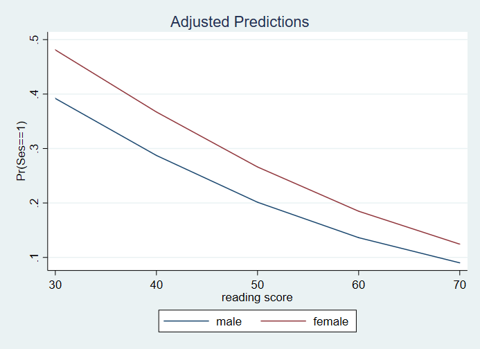
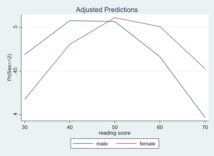
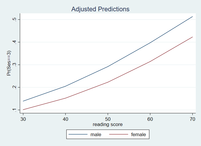
Please note: The values in the tables and graphs above are predicted probabilities. The column heading for the margins tables, Coef., is incorrect.
In case you lose track of which values in the margins output are which, you can list the r(at) matrix.
matrix list r(at)

r(at)[10,3]
           female       read       math
 1._at          0         30  51.691358
 2._at          0         40  51.691358
 3._at          0         50  51.691358
 4._at          0         60  51.691358
 5._at          0         70  51.691358
 6._at          1         30  51.691358
 7._at          1         40  51.691358
 8._at          1         50  51.691358
 9._at          1         60  51.691358
10._at          1         70  51.691358
This may not be the most transparent process ever but, in the end, we got the plots of the predicted probabilities. Of course, the technique shown here is not restricted to ologit but generalizes to many other estimation procedures for use with margins and marginsplot.
Acknowledgements
Thanks to Isabel Cannette of Stata Corp for the suggestion to use myret to repost the margins results.