It is fairly easy to generate power curves for the chi-square distribution using Stata. This FAQ page will show you one way you can do it. Here is a code fragment that you can paste into you do-file editor and run. We’ll talk about it after you take a look at it. Please note that you can change the graph scheme to a different one if you don’t care for lean1.
drop _all
local df = 1
range ncp 0 40 201
foreach a of numlist 1 5 10 50 {
  local alpha=`a'/100
  local cv = invchi2(`df', 1-`alpha')
  generate p`a' = 1-nchi2(`df', ncp, `cv')
}
twoway (line p1 p5 p10 p50 ncp, yline(.8)), legend(order(1 ".01" 2 ".05" 3 ".10" 4 ".50")) ///
       t2title("power curves for chi-square (df=`df')") aspect(.9) scheme(lean1)
In the code fragment above the range command generates the values of the noncentrality parameter, ncp (which we will talk about below), which ranges from 0 to 40 in steps of 0.2. The foreach loop steps through each of the four values to be used as the alpha levels, .01, .05, .10, and .50. The invchi2() function is used to get the critical value of the central chi-square distribution, i.e., the distribution if chi-square under the null hypothesis. To show you how this function works, we will run it manually from the command line.
display invchi2(1, 1-.05)

3.8414588
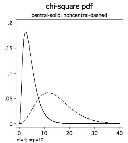
You might recognize that value, 3.84 as the critical value of chi-square for alpha equal 0.05 with one degree of freedom. There is another chi-square function, nchi2(), which computes the probabilities for the noncentral chi-square distribution, that is, the distribution of chi-square under the alternative hypothesis. The noncentrality parameter (ncp) indicates how different the noncentral distribution is from the central distribution. The larger the ncp the greater the difference from the central chi-square distribution. Relative to the central chi-square distribution the noncentral distribution is shifted to the right and has greater variability as shown in the figure below with degrees of freedom equal 6 and ncp equal to 10.
The noncentral chi-square function, nchi2(), requires both a critical value of chi-square and a noncentrality parameter. The trick to computing power for chi-square is to use the critical value from the central chi-square distribution along with a noncentrality parameter from a noncentral chi-square distribution to compute the probability of rejecting the null hypothesis when it is false.
So now we can go ahead and run the program and look at the graph it produces.
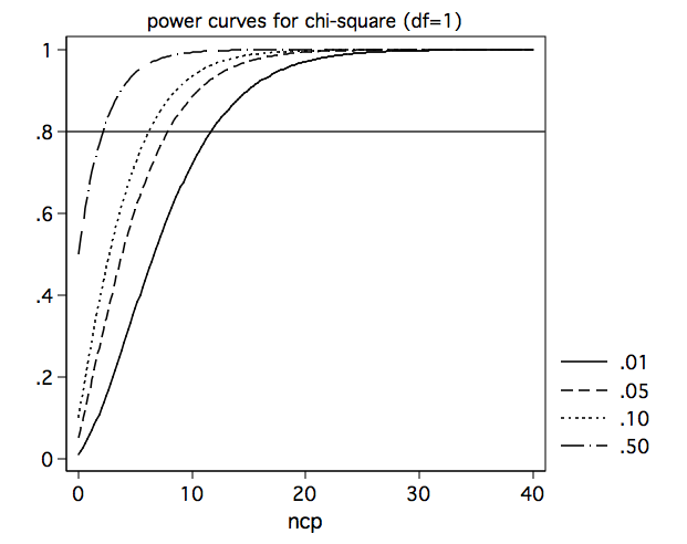
The power curves show that power increases as the nocentrality parameter increases and power decreases as alpha gets smaller. This is exactly the way you would expect power to behave.
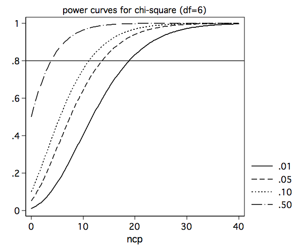
If you change the value of df in the third line of the program to 6, you will get the power curves for six degrees of freedom.
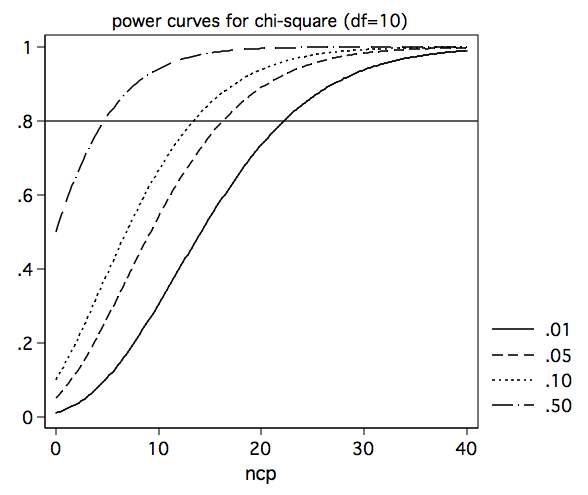
And if we change df to 10, we get the following set of curves.
Now, let’s see how you might be able to make use of this information. To illustrate this we will download the hsblog dataset and run a logistic regression. By the way, it is just a coincidence that there are 200 observations in the hsblog dataset and 200 data points used in the plotting of the power curves.
use https://stats.idre.ucla.edu/stat/data/hsblog, clear

logit honcomp female, nolog

Logistic regression                               Number of obs   =        200
                                                  LR chi2(1)      =       3.94
                                                  Prob > chi2     =     0.0473
Log likelihood =  -113.6769                       Pseudo R2       =     0.0170

------------------------------------------------------------------------------
     honcomp |      Coef.   Std. Err.      z    P>|z|     [95% Conf. Interval]
-------------+----------------------------------------------------------------
      female |   .6513707   .3336752     1.95   0.051    -.0026207    1.305362
       _cons |  -1.400088   .2631619    -5.32   0.000    -1.915876   -.8842998
------------------------------------------------------------------------------
We can use the likelihood ratio chi-square value (3.94) as an estimate of the noncentrality parameter with one degree of freedom. We will also note that the p-value is 0.0473 which is very close to our alpha level of 0.05. Next we will rerun the code fragment above setting the df back to one. After the program runs, list ncp and p5 (p5 is the name of the variable that contains the power for alpha equal to 0.05).
clist ncp p5 in 1/25

           ncp         p5
  1.         0        .05
  2.        .2   .0732097
  3.        .4   .0969355
  4.        .6   .1210593
  5.        .8   .1454725
  6.         1    .170075
  7.       1.2   .1947752
  8.       1.4   .2194893
  9.       1.6   .2441412
 10.       1.8   .2686618
 11.         2   .2929889
 12.       2.2   .3170667
 13.       2.4   .3408451
 14.       2.6     .36428
 15.       2.8   .3873324
 16.         3   .4099681
 17.       3.2   .4321576
 18.       3.4   .4538757
 19.       3.6   .4751009
 20.       3.8   .4958155
 21.         4   .5160053
 22.       4.2   .5356588
 23.       4.4   .5547677
 24.       4.6   .5733261
 25.       4.8   .5913305
Our estimate of the noncentrality parameter was 3.94 which falls between 3.8 and 4.0 in the above listing with power falling between .4958155 and .5160053, i.e., a power of approximately .5 which is about what we would expect with an alpha of approximately 0.05.
Let’s try one more example, this time using a two degree of freedom test.
use https://stats.idre.ucla.edu/stat/data/hsblog, clear

logit honcomp i.prog, nolog

Logistic regression                             Number of obs     =        200
                                                LR chi2(2)        =      16.15
                                                Prob > chi2       =     0.0003
Log likelihood =  -107.5719                     Pseudo R2         =     0.0698

------------------------------------------------------------------------------
     honcomp |      Coef.   Std. Err.      z    P>|z|     [95% Conf. Interval]
-------------+----------------------------------------------------------------
        prog |
   academic  |   1.206168   .4577746     2.63   0.008     .3089465     2.10339
   vocation  |  -.3007541   .5988045    -0.50   0.615    -1.474389    .8728812
             |
       _cons |  -1.691676   .4113064    -4.11   0.000    -2.497822   -.8855303
------------------------------------------------------------------------------
We will need to run the code fragment one more time setting the df to 2 then we can list the results for a range of ncp values.
clist ncp p5 if ncp>15.5 & ncp<17.5

           ncp         p5
 79.      15.6   .9519728
 80.      15.8   .9543857
 81.        16   .9566863
 82.      16.2   .9588793
 83.      16.4   .9609691
 84.      16.6   .9629601
 85.      16.8   .9648565
 86.        17   .9666622
 87.      17.2   .9683813
 88.      17.4   .9700173
Using the likelihood ratio chi-square of 16.15 as the ncp estimate we see that the estimated power falls between .9566863 and .9588793, which again seems reasonable given the very small p-value.
Please note that we are not advocating post-hoc power analysis with these two examples; rather, we are just demonstrating how the power curves work.