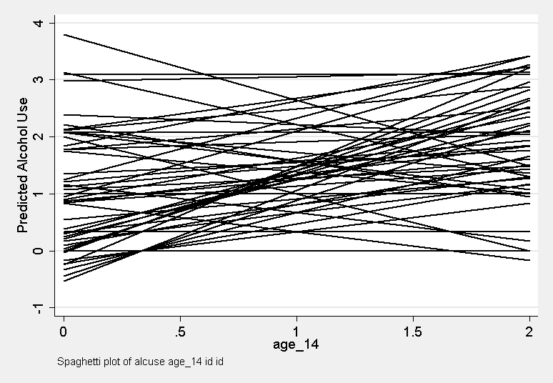
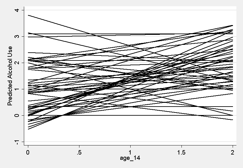
ATS has created a program called spagplot to help you easily produce spaghetti plots using Stata. You can install spagplot over the internet by typing search spagplot (see How can I used the search command to search for programs and get additional help? for more information about using search).
NOTE! Spagplot makes the assumption that the first X variable for subject i+1 is less than the last X variable for subject "i" and this is not always true. When this is flase, the lines for two subjects will get connected.
The syntax of spagplot is
spagplot yvar xvar [if exp] [in range], id(idvar) [graph options]
We will show a number of examples from a data file which contains alcohol use alcuse at 3 ages, age 14, 15, and 16 for a number of children (identified by the variable id). The age variable has been centered around age 14 and is named age_14. We first show how to obtain the data file.
use https://stats.idre.ucla.edu/stat/stata/examples/alda/data/alcohol1_pp, clear
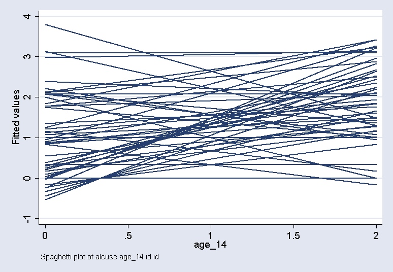
This example shows a basic spaghetti plot of alcohol use by age, broken down by id.
spagplot alcuse age_14 , id( id )
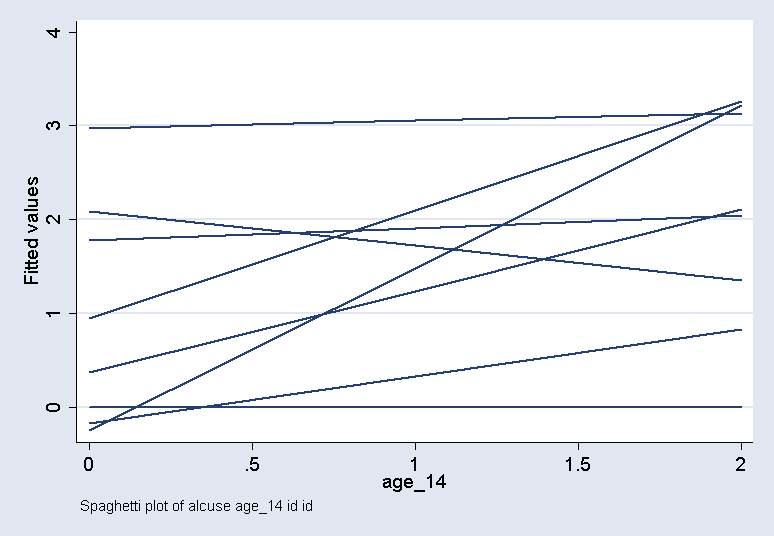
This example just performs the plot for the first 30 observations in the file.
spagplot alcuse age_14 in 1/30, id( id )
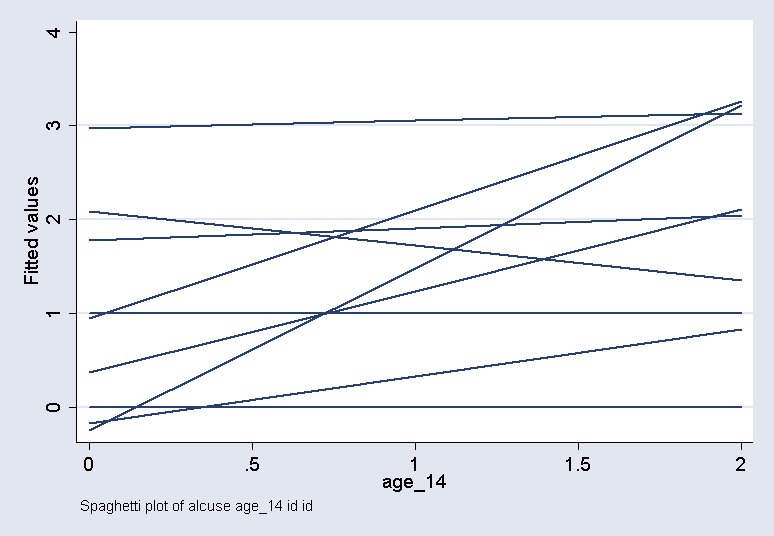
This example shows the plot just for the ids below 9.
spagplot alcuse age_14 if id <= 9, id( id )
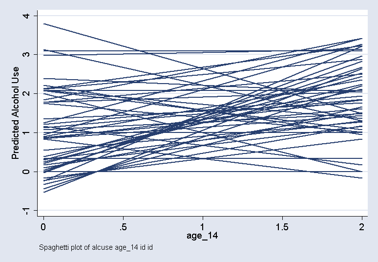
This example adds a title as a graph option.
spagplot alcuse age_14 , id( id ) ytitle("Predicted Alcohol Use")
This example adds a title as a graph option, and changes the scheme to sj.
spagplot alcuse age_14 , id( id ) ytitle("Predicted Alcohol Use") scheme(sj)
This example also changes the note from the default note.
spagplot alcuse age_14 , id( id ) ytitle("Predicted Alcohol Use") scheme(sj) note("My custom note")
This example removes the note from the graph entirely.
spagplot alcuse age_14 , id( id ) ytitle("Predicted Alcohol Use") scheme(sj) note("")

