Testing simple effects in repeated measures models that have both between-subjects and within-subjects effects can be tricky. We will look at two different estimation approaches, linear mixed model and anova. The example we will use is a split-plot factorial with a two-level between variable (a) and a four-level within variable (b). There are four subjects at each level of a.
We begin by loading the data and producing some descriptive statistics.
use https://stats.idre.ucla.edu/stat/data/spf24, clear

tab1 a b s

-> tabulation of a

          a |      Freq.     Percent        Cum.
------------+-----------------------------------
          1 |         16       50.00       50.00
          2 |         16       50.00      100.00
------------+-----------------------------------
      Total |         32      100.00

-> tabulation of b

          b |      Freq.     Percent        Cum.
------------+-----------------------------------
          1 |          8       25.00       25.00
          2 |          8       25.00       50.00
          3 |          8       25.00       75.00
          4 |          8       25.00      100.00
------------+-----------------------------------
      Total |         32      100.00

-> tabulation of s

          s |      Freq.     Percent        Cum.
------------+-----------------------------------
          1 |          4       12.50       12.50
          2 |          4       12.50       25.00
          3 |          4       12.50       37.50
          4 |          4       12.50       50.00
          5 |          4       12.50       62.50
          6 |          4       12.50       75.00
          7 |          4       12.50       87.50
          8 |          4       12.50      100.00
------------+-----------------------------------
      Total |         32      100.00

tabstat y, by(a)

Summary for variables: y
     by categories of: a

       a |      mean
---------+----------
       1 |    5.6875
       2 |    5.0625
---------+----------
   Total |     5.375
--------------------

tabstat y, by(a)

Summary for variables: y
     by categories of: a

       a |      mean
---------+----------
       1 |    5.6875
       2 |    5.0625
---------+----------
   Total |     5.375
--------------------

egen ab=group(a b), label

tabstat y, by(ab)

Summary for variables: y
     by categories of: ab (group(a b))

    ab |      mean
-------+----------
   1 1 |      3.75
   1 2 |         4
   1 3 |         7
   1 4 |         8
   2 1 |      1.75
   2 2 |         3
   2 3 |       5.5
   2 4 |        10
-------+----------
 Total |     5.375
------------------
Let’s begin with a linear mixed model using the mixed command. We will need to specify the reml option so that the results are consistent with the anova command that we will run later. Starting with Stata 12 the default estimation method is mle, which is why we need to specify the reml option.
mixed y a##b || s:, reml stddev


Performing EM optimization:

Performing gradient-based optimization:

Iteration 0:   log restricted-likelihood = -34.824381
Iteration 1:   log restricted-likelihood = -34.824379

Computing standard errors:

Mixed-effects REML regression                   Number of obs      =        32
Group variable: s                               Number of groups   =         8

                                                Obs per group: min =         4
                                                               avg =       4.0
                                                               max =         4


                                                Wald chi2(7)       =    423.89
Log restricted-likelihood = -34.824379          Prob > chi2        =    0.0000

------------------------------------------------------------------------------
           y |      Coef.   Std. Err.      z    P>|z|     [95% Conf. Interval]
-------------+----------------------------------------------------------------
         2.a |         -2   .6208193    -3.22   0.001    -3.216783   -.7832165
             |
           b |
          2  |        .25   .5034603     0.50   0.619     -.736764    1.236764
          3  |       3.25   .5034603     6.46   0.000     2.263236    4.236764
          4  |       4.25   .5034603     8.44   0.000     3.263236    5.236764
             |
         a#b |
        2 2  |          1   .7120004     1.40   0.160    -.3954951    2.395495
        2 3  |         .5   .7120004     0.70   0.483    -.8954951    1.895495
        2 4  |          4   .7120004     5.62   0.000     2.604505    5.395495
             |
       _cons |       3.75   .4389855     8.54   0.000     2.889604    4.610396
------------------------------------------------------------------------------

------------------------------------------------------------------------------
  Random-effects Parameters  |   Estimate   Std. Err.     [95% Conf. Interval]
-----------------------------+------------------------------------------------
s: Identity                  |
                   sd(_cons) |    .513701   .2233302      .2191052    1.204393
-----------------------------+------------------------------------------------
                sd(Residual) |   .7120004   .1186667      .5135861    .9870682
------------------------------------------------------------------------------
LR test vs. linear regression: chibar2(01) =     3.30 Prob >= chibar2 = 0.0346

contrast a##b /* test main effects and interaction */

Contrasts of marginal linear predictions

Margins: asbalanced

------------------------------------------------
             |         df        chi2     P>chi2
-------------+----------------------------------
y            |
           a |          1        2.00     0.1573
             |
           b |          3      383.67     0.0000
             |
         a#b |          3       38.22     0.0000
------------------------------------------------
The results above indicate that the a main effect is not significant. Both the b main effect and the a#b interaction are significant.
The results of the contrast displayed are displayed as chi-square. We will divide each chi-square by its degrees of freedom so that the results are scaled as F-ratios (we will not do the division when df=1).
/* scale as F-ratio*/

display 383.67/3

127.89

display 38.22/3
12.74
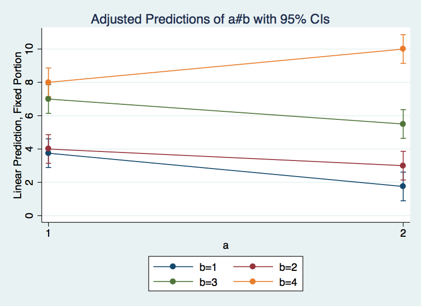
Next, we will run the margins command followed by marginsplot so that we can plot the interaction.
margins a#b, vsquish Adjusted predictions Number of obs = 32
Expression: Linear prediction, fixed portion, predict()
------------------------------------------------------------------------------
| Delta-method
| Margin std. err. z P>|z| [95% conf. interval]
-------------+----------------------------------------------------------------
a#b |
1 1 | 3.75 .4389855 8.54 0.000 2.889604 4.610396
1 2 | 4 .4389855 9.11 0.000 3.139604 4.860396
1 3 | 7 .4389855 15.95 0.000 6.139604 7.860396
1 4 | 8 .4389855 18.22 0.000 7.139604 8.860396
2 1 | 1.75 .4389855 3.99 0.000 .8896042 2.610396
2 2 | 3 .4389855 6.83 0.000 2.139604 3.860396
2 3 | 5.5 .4389855 12.53 0.000 4.639604 6.360396
2 4 | 10 .4389855 22.78 0.000 9.139604 10.8604
------------------------------------------------------------------------------
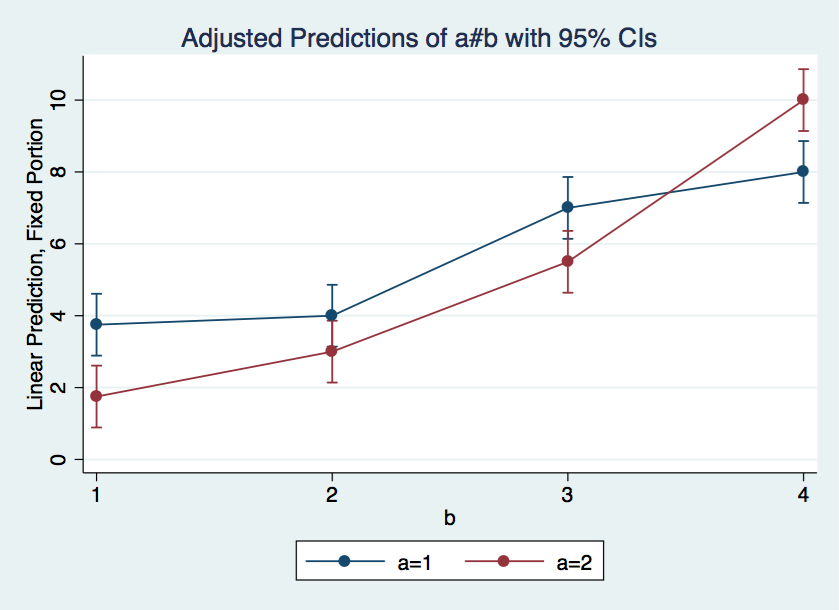
marginsplot
 marginsplot, x(b)
At last we are ready to look at the tests of simple effects. We will look at both a for each level of b and for b at each level of a. These computations will be done using the contrast command. Running contrast after mixed displays the results as chi-square. We will divide each of the chi-square values by its degrees of freedom to scale the results as a F-ratio, for later comparison to our anova results.
contrast a@b  // simple effects for a at each level of b

Contrasts of marginal linear predictions

Margins      : asbalanced

------------------------------------------------
             |         df        chi2     P>chi2
-------------+----------------------------------
y            |
         a@b |
          1  |          1       10.38     0.0013
          2  |          1        2.59     0.1072
          3  |          1        5.84     0.0157
          4  |          1       10.38     0.0013
      Joint  |          4       40.22     0.0000
------------------------------------------------

contrast b@a  /* simple effects for b at each level of a */  Contrasts of marginal linear predictions

Margins: asbalanced

------------------------------------------------
             |         df        chi2     P>chi2
-------------+----------------------------------
y            |
         b@a |
          1  |          3      107.88     0.0000
          2  |          3      314.01     0.0000
      Joint  |          6      421.89     0.0000
------------------------------------------------

/* scale as F-ratio */ display 107.88/3

35.96

display 314.01/3

104.67
The raw p-values for a@b indicate that a at b1, b3 and b4 are significant. For, b@a both simple effects are significant using the raw p-values. Test of simple effects are a type of post-hoc procedure and need to be adjusted. We won’t go into the adjustment process on this page other than to state that there are at least four methods found in the literature (Dunn’s procedure, Marascuilo & Levin, per family error rate or simultaneous test procedure).
Next we will use the anova command to analyze the repeated measures model.
anova y a / s|a b a#b, repeated(b)


                           Number of obs =      32     R-squared     =  0.9613
                           Root MSE      =    .712     Adj R-squared =  0.9333

                  Source |  Partial SS    df       MS           F     Prob > F
              -----------+----------------------------------------------------
                   Model |     226.375    13  17.4134615      34.35     0.0000
                         |
                       a |       3.125     1       3.125       2.00     0.2070
                     s|a |       9.375     6      1.5625
              -----------+----------------------------------------------------
                       b |       194.5     3  64.8333333     127.89     0.0000
                     a#b |      19.375     3  6.45833333      12.74     0.0001
                         |
                Residual |       9.125    18  .506944444
              -----------+----------------------------------------------------
                   Total |       235.5    31  7.59677419


Between-subjects error term:  s|a
                     Levels:  8         (6 df)
     Lowest b.s.e. variable:  s
     Covariance pooled over:  a         (for repeated variable)

Repeated variable: b
                                          Huynh-Feldt epsilon        =  0.9432
                                          Greenhouse-Geisser epsilon =  0.5841
                                          Box's conservative epsilon =  0.3333

                                            ------------ Prob > F ------------
                  Source |     df      F    Regular    H-F      G-G      Box
              -----------+----------------------------------------------------
                       b |      3   127.89   0.0000   0.0000   0.0000   0.0000
                     a#b |      3    12.74   0.0001   0.0002   0.0019   0.0118
                Residual |     18
              ----------------------------------------------------------------
The results in the anova table above agree with results from mixed once the chi-squares have been rescaled as F-ratios. Computing the simple effects after the anova is a more complex process than we used above. One reason for this is that the two types of simple effects, a@b and b@a, involve different error terms.
Let’s start with a@b. The sums of square for simple effects for a@b total up to SSa + SSa#b. The test of a uses s|a as the error term while test of a#b use the residual. The recommendation for testing simple effects for a@b are to pool s|a and residual. We can accomplish this by running the anova without the s|a term. After the anova we will use the contrast command to get the simple effects.
anova y a b a#b


                           Number of obs =      32     R-squared     =  0.9214
                           Root MSE      = .877971     Adj R-squared =  0.8985

                  Source |  Partial SS    df       MS           F     Prob > F
              -----------+----------------------------------------------------
                   Model |         217     7          31      40.22     0.0000
                         |
                       a |       3.125     1       3.125       4.05     0.0554
                       b |       194.5     3  64.8333333      84.11     0.0000
                     a#b |      19.375     3  6.45833333       8.38     0.0006
                         |
                Residual |        18.5    24  .770833333
              -----------+----------------------------------------------------
                   Total |       235.5    31  7.59677419


contrast a@b

Contrasts of marginal linear predictions

Margins      : asbalanced

------------------------------------------------
             |         df           F        P>F
-------------+----------------------------------
         a@b |
          1  |          1       10.38     0.0036
          2  |          1        2.59     0.1203
          3  |          1        5.84     0.0237
          4  |          1       10.38     0.0036
      Joint  |          4        7.30     0.0005
             |
    Residual |         24
------------------------------------------------
Once again the F-values are the same for this analysis as for the contrast command used in the mixed analysis. You will note that the p-values are different. The p-values above are from an F-distribution with 1 and 24 degrees of freedom. The p-values from the mixed analysis are distributed as a chi-square with 1 degree of freedom.
Now we need to compute the simple effects for b@a. To do this we will quietly rerun the anova model followed by the margins command with the within option to see what our cell means are.
quietly anova y a / s|a b a#b

margins b, within(a)

Predictive margins                                Number of obs   =         32

Expression   : Linear prediction, predict()
within       : a
Empty cells  : reweight

------------------------------------------------------------------------------
             |            Delta-method
             |     Margin   Std. Err.      z    P>|z|     [95% Conf. Interval]
-------------+----------------------------------------------------------------
         a#b |
        1 1  |       3.75   .3560002    10.53   0.000     3.052253    4.447747
        1 2  |          4   .3560002    11.24   0.000     3.302253    4.697747
        1 3  |          7   .3560002    19.66   0.000     6.302253    7.697747
        1 4  |          8   .3560002    22.47   0.000     7.302253    8.697747
        2 1  |       1.75   .3560002     4.92   0.000     1.052253    2.447747
        2 2  |          3   .3560002     8.43   0.000     2.302253    3.697747
        2 3  |        5.5   .3560002    15.45   0.000     4.802253    6.197747
        2 4  |         10   .3560002    28.09   0.000     9.302253    10.69775
------------------------------------------------------------------------------
We will compute the simple effects of b@a using the contrast command.
>contrast b@a Contrasts of marginal linear predictions

Margins: asbalanced

------------------------------------------------
             |         df           F        P>F
-------------+----------------------------------
         b@a |
          1  |          3       35.96     0.0000
          2  |          3      104.67     0.0000
      Joint  |          6       70.32     0.0000
             |
 Denominator |         18
------------------------------------------------
Once again, our results from the anova agree with the results for the mixed. We see that each of the tests of simple effects are distributed as F with 3 and 18 degrees of freedom. We also note that the results agree with the mixed results above once they are scaled from chi-square to F-ratios.
At this point, it would be nice to run pairwise comparisons among each of the levels of b at each level of a. We can do this using the pwcompare command. We want the pairwise comparisons adjusted using Tudkey’s HSD. We get this using the mcompare option. Please note that you cannot get the Tukey adjustment from mixed models.
/* pairwise comparisons for a = 1 */

pwcompare b#i(1).a, mcompare(tukey) effects

Pairwise comparisons of marginal linear predictions

Margins      : asbalanced

---------------------------
             |    Number of
             |  Comparisons
-------------+-------------
         b#a |            6
---------------------------

---------------------------------------------------------------------------------
                |                              Tukey                Tukey
                |   Contrast   Std. Err.      t    P>|t|     [95% Conf. Interval]
----------------+----------------------------------------------------------------
            b#a |
(2 1) vs (1 1)  |        .25   .5034602     0.50   0.959    -1.172925    1.672925
(3 1) vs (1 1)  |       3.25   .5034602     6.46   0.000     1.827075    4.672925
(4 1) vs (1 1)  |       4.25   .5034602     8.44   0.000     2.827075    5.672925
(3 1) vs (2 1)  |          3   .5034602     5.96   0.000     1.577075    4.422925
(4 1) vs (2 1)  |          4   .5034602     7.95   0.000     2.577075    5.422925
(4 1) vs (3 1)  |          1   .5034602     1.99   0.230    -.4229247    2.422925
---------------------------------------------------------------------------------

/* pairwise comparisons for a = 2 */

pwcompare b#i(2).a, mcompare(tukey) effects

Pairwise comparisons of marginal linear predictions

Margins      : asbalanced

---------------------------
             |    Number of
             |  Comparisons
-------------+-------------
         b#a |            6
---------------------------

---------------------------------------------------------------------------------
                |                              Tukey                Tukey
                |   Contrast   Std. Err.      t    P>|t|     [95% Conf. Interval]
----------------+----------------------------------------------------------------
            b#a |
(2 2) vs (1 2)  |       1.25   .5034602     2.48   0.097    -.1729247    2.672925
(3 2) vs (1 2)  |       3.75   .5034602     7.45   0.000     2.327075    5.172925
(4 2) vs (1 2)  |       8.25   .5034602    16.39   0.000     6.827075    9.672925
(3 2) vs (2 2)  |        2.5   .5034602     4.97   0.001     1.077075    3.922925
(4 2) vs (2 2)  |          7   .5034602    13.90   0.000     5.577075    8.422925
(4 2) vs (3 2)  |        4.5   .5034602     8.94   0.000     3.077075    5.922925
---------------------------------------------------------------------------------
Reference
Kirk, Roger E. (1995) Experimental Design: Procedures for the Behavioral Sciences, Third Edition. Monterey, California: Brooks/Cole Publishing.