Interactions in logistic regression models can be trickier than interactions in comparable OLS regression models. This is particularly true when there are covariates in the model in addition to the categorical predictors. This FAQ page will try to help you to understand categorical by categorical interactions in logistic regression models with continuous covariates.
We will use an example dataset, logit2-2, that has two binary predictors, f and h, and a continuous covariate, cv1. In addition, the model will include f by h interaction. We will begin by loading the data, creating the interaction variable and running the logit model.
use https://stats.idre.ucla.edu/stat/data/logit2-2, clear

logit y f##h cv1

Logistic regression                               Number of obs   =        200
                                                  LR chi2(4)      =     106.10
                                                  Prob > chi2     =     0.0000
Log likelihood =  -78.74193                       Pseudo R2       =     0.4025

------------------------------------------------------------------------------
           y |      Coef.   Std. Err.      z    P>|z|     [95% Conf. Interval]
-------------+----------------------------------------------------------------
         1.f |   2.996118   .7521524     3.98   0.000     1.521926    4.470309
         1.h |   2.390911   .6608498     3.62   0.000      1.09567    3.686153
             |
         f#h |
        1 1  |  -2.047755   .8807989    -2.32   0.020    -3.774089   -.3214213
             |
         cv1 |    .196476   .0328518     5.98   0.000     .1320876    .2608644
       _cons |  -11.86075   1.895828    -6.26   0.000     -15.5765   -8.144991
------------------------------------------------------------------------------
As you can see all of the variables in the above model including the interaction term are statistically significant. If this were an OLS regression model we could do a very good job of understanding the interaction using just the coefficients in the model. The situation in logistic regression is more complicated because the effect of the covariate is nonlinear, meaning that the interaction effect can be very different for different values of the covariate. To begin to understand what is going on consider the Table 1 below.
Table 1: Predicted probabilities when cv1=50

        h=0     h=1    Dprob      LB       UB
f=0   .1154   .5876   .4722    .2693    .6751
f=1   .7230   .7862   .0633   -.1399    .2665
Table 1 contain predicted probabilities, differences in predicted probabilities and the confidence interval of the difference in predicted probabilities while holding cv1 at 50. The first value, .1154, is the predicted probability when f=0 and h=0. The second value, .5876, is the predicted probability when f=0 and h=1. The third value, .4722, is the difference in probabilities for f=0 when h changes from 0 to 1. The next two values are the 95% confidence interval on the difference in probabilities. If the confidence interval contains zero the difference would not be considered statistically significant. In our example, the confidence interval does not contain zero. Thus, for our example, the difference in probabilities is statistically significant.
We we can obtained all the values for Table 1 for a range of values of cv1 by using the margins command twice. We run margins once to get the probabilities for h = 0 and h = 1 for both f equal 0 and 1.
margins h, at(f=(0 1) cv1=(30(5)70)) vsquish

Adjusted predictions                              Number of obs   =        200
Model VCE    : OIM

Expression   : Pr(y), predict()
1._at        : f               =           0
               cv1             =          30
2._at        : f               =           0
               cv1             =          35
3._at        : f               =           0
               cv1             =          40
4._at        : f               =           0
               cv1             =          45
5._at        : f               =           0
               cv1             =          50
6._at        : f               =           0
               cv1             =          55
7._at        : f               =           0
               cv1             =          60
8._at        : f               =           0
               cv1             =          65
9._at        : f               =           0
               cv1             =          70
10._at       : f               =           1
               cv1             =          30
11._at       : f               =           1
               cv1             =          35
12._at       : f               =           1
               cv1             =          40
13._at       : f               =           1
               cv1             =          45
14._at       : f               =           1
               cv1             =          50
15._at       : f               =           1
               cv1             =          55
16._at       : f               =           1
               cv1             =          60
17._at       : f               =           1
               cv1             =          65
18._at       : f               =           1
               cv1             =          70

------------------------------------------------------------------------------
             |            Delta-method
             |     Margin   Std. Err.      z    P>|z|     [95% Conf. Interval]
-------------+----------------------------------------------------------------
       _at#h |
        1 0  |   .0025567   .0025254     1.01   0.311    -.0023929    .0075063
        1 1  |   .0272372   .0206496     1.32   0.187    -.0132352    .0677097
        2 0  |   .0067995   .0057853     1.18   0.240    -.0045396    .0181385
        2 1  |    .069579   .0413211     1.68   0.092    -.0114088    .1505668
        3 0  |   .0179561   .0129716     1.38   0.166    -.0074678      .04338
        3 1  |   .1664783   .0709412     2.35   0.019     .0274362    .3055204
        4 0  |   .0465604    .028158     1.65   0.098    -.0086283     .101749
        4 1  |   .3478701   .0933387     3.73   0.000     .1649296    .5308105
        5 0  |    .115378   .0575106     2.01   0.045     .0026592    .2280968  value from Table 1
        5 1  |   .5875788   .0877652     6.69   0.000     .4155621    .7595955  value from Table 1
        6 0  |   .2583492   .1025789     2.52   0.012     .0572982    .4594002
        6 1  |   .7918883   .0631887    12.53   0.000     .6680407    .9157359
        7 0  |   .4819613   .1389465     3.47   0.001      .209631    .7542915
        7 1  |    .910416    .037977    23.97   0.000     .8359824    .9848496
        8 0  |   .7130398   .1272483     5.60   0.000     .4636377    .9624418
        8 1  |   .9644667   .0200004    48.22   0.000     .9252666    1.003667
        9 0  |   .8690487   .0818878    10.61   0.000     .7085515    1.029546
        9 1  |   .9863932   .0096629   102.08   0.000     .9674543    1.005332
       10 0  |   .0487835   .0294567     1.66   0.098    -.0089504    .1065175
       10 1  |   .0674087   .0446964     1.51   0.132    -.0201947    .1550121
       11 0  |   .1204719   .0549249     2.19   0.028     .0128212    .2281227
       11 1  |   .1618113     .07791     2.08   0.038     .0091104    .3145121
       12 0  |    .267844   .0851192     3.15   0.002     .1010134    .4346747
       12 1  |   .3401934   .1024706     3.32   0.001     .1393547    .5410321
       13 0  |   .4941981   .1006298     4.91   0.000     .2969673    .6914289
       13 1  |   .5793115   .0914477     6.33   0.000     .4000773    .7585456
       14 0  |   .7229559   .0872338     8.29   0.000     .5519808    .8939309  value from Table 1
       14 1  |   .7862264   .0599327    13.12   0.000     .6687605    .9036924  value from Table 1
       15 0  |   .8745225   .0571538    15.30   0.000      .762503     .986542
       15 1  |   .9076026    .034318    26.45   0.000     .8403406    .9748645
       16 0  |   .9490168   .0308608    30.75   0.000     .8885308    1.009503
       16 1  |   .9632823   .0180954    53.23   0.000     .9278159    .9987487
       17 0  |   .9802821   .0149266    65.67   0.000     .9510265    1.009538
       17 1  |    .985929   .0088829   110.99   0.000     .9685188    1.003339
       18 0  |    .992525    .006799   145.98   0.000     .9791993    1.005851
       18 1  |   .9946848   .0041367   240.46   0.000      .986577    1.002792
------------------------------------------------------------------------------
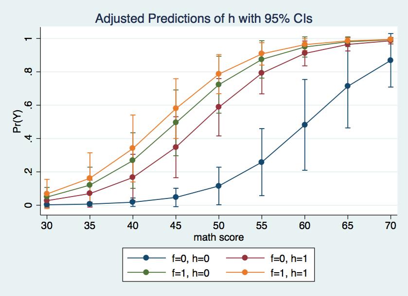
Using the marginsplot command we can graph the predicted probabilities for each of the four cells in the design for various values of the covariate.
marginsplot, x(cv1)

The graph above shows the f = 0, h = 0 cell is rather different from the other three cells.
Next, we will run margins again to get the difference in probabilities and them confidence interval for the difference. We will manually annotate the output to indicate which values are the same as Table 1.
margins f, dydx(h) at(cv1=(30(5)70)) vsquish

Conditional marginal effects                      Number of obs   =        200
Model VCE    : OIM

Expression   : Pr(y), predict()
dy/dx w.r.t. : 1.h
1._at        : cv1             =          30
2._at        : cv1             =          35
3._at        : cv1             =          40
4._at        : cv1             =          45
5._at        : cv1             =          50
6._at        : cv1             =          55
7._at        : cv1             =          60
8._at        : cv1             =          65
9._at        : cv1             =          70

------------------------------------------------------------------------------
             |            Delta-method
             |      dy/dx   Std. Err.      z    P>|z|     [95% Conf. Interval]
-------------+----------------------------------------------------------------
1.h          |
       _at#f |
        1 0  |   .0246805   .0188412     1.31   0.190    -.0122475    .0616086
        1 1  |   .0186252   .0331697     0.56   0.574    -.0463863    .0836367
        2 0  |   .0627795   .0378532     1.66   0.097    -.0114115    .1369704
        2 1  |   .0413394   .0695885     0.59   0.552    -.0950517    .1777304
        3 0  |   .1485222   .0656193     2.26   0.024     .0199107    .2771337
        3 1  |   .0723494   .1167547     0.62   0.535    -.1564856    .3011843
        4 0  |   .3013097   .0902579     3.34   0.001     .1244074     .478212
        4 1  |   .0851134   .1360832     0.63   0.532    -.1816048    .3518315
        5 0  |   .4722008   .1035128     4.56   0.000     .2693194    .6750821  value from Table 1
        5 1  |   .0632706   .1036697     0.61   0.542    -.1399183    .2664595  value from Table 1
        6 0  |   .5335391   .1208833     4.41   0.000     .2966122    .7704659
        6 1  |   .0330801   .0565538     0.58   0.559    -.0777632    .1439234
        7 0  |   .4284548    .137549     3.11   0.002     .1588636    .6980459
        7 1  |   .0142654   .0255894     0.56   0.577    -.0358888    .0644197
        8 0  |   .2514269    .120641     2.08   0.037      .014975    .4878788
        8 1  |   .0056469   .0106397     0.53   0.596    -.0152065    .0265003
        9 0  |   .1173445    .076704     1.53   0.126    -.0329926    .2676816
        9 1  |   .0021597   .0042758     0.51   0.613    -.0062207    .0105402
------------------------------------------------------------------------------
Note: dy/dx for factor levels is the discrete change from the base level.
Here is what we can say based upon the output above. There are no significant differences between the two levels of h when the covariate is held constant at either 30 or 35. When the covariate is held constant between 40 and 65 there is a significant h 0-1 difference at f=0 but not at f=1. Finally, when the covariates are held constant at 70 the h differences are not significant. It may be easier to understand these results if we graph the confidence intervals for the difference in probability separately for both f=0 and f=1.
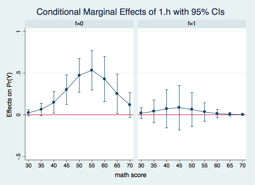
There is so much information in the margins output that its difficult to see what is going on. A graphic representation would do a better job of organizing and displaying the results. We will produce the graphs using using the marginsplot command once again.
marginsplot, x(cv1) by(f) yline(0)
Wherever the confidence interval includes zero the differences in the adjusted probabilities between h = 0 and h = 1 is not statistically significant. This is the case for all of the data points in the graph for f = 1. On the other hand, for f = 0, all of the differences in probabilities between cv1 = 40 and 65 appear to be significant.
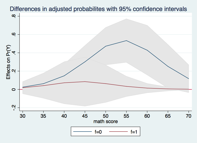
Finally, we will try to combine the two halves of the graph into a single graph with shaded confidence intervals. There is no new information here, we are just aiming at a more visually interesting graph.
marginsplot, recast(line) recastci(rarea) ciopts(color(gs14)) x(cv1) yline(0) ///
             title(Differences in adjusted probabilites with 95% confidence intervals)


