The techniques and methods for this FAQ page were drawn from the work of Long (2006) and Hu & Long (2005).
Interactions in logistic regression models can be trickier than interactions in comparable OLS regression.
Many researchers are not comfortable interpreting the results in terms of the raw coefficients which are scaled in terms of log odds. The interpretation of interactions in log odds is done basically the same way as in OLS regression. However, many researchers prefer to interpret results in terms of probabilities. The shift from log odds to probabilities is a nonlinear transformation which means that the interactions are no longer a simple linear function of the predictors. This FAQ page will try to help you to understand categorical by continuous interactions in logistic regression models both with and without covariates.
We will use an example dataset, logitcatcon, that has one binary predictor, f, which stands for female and one continuous predictor s. In addition, the model will include fs which is the f by s interaction. We will begin by loading the data, creating the interaction variable and running the logit model.
use https://stats.idre.ucla.edu/stat/data/logitcatcon, clear

generate fs = f*s

logit y f s fs, nolog

Logistic regression                               Number of obs   =        200
                                                  LR chi2(3)      =      71.01
                                                  Prob > chi2     =     0.0000
Log likelihood =  -96.28586                       Pseudo R2       =     0.2694

------------------------------------------------------------------------------
           y |      Coef.   Std. Err.      z    P>|z|     [95% Conf. Interval]
-------------+----------------------------------------------------------------
           f |   5.786811   2.302491     2.51   0.012     1.274012    10.29961
           s |   .1773383   .0364356     4.87   0.000     .1059259    .2487507
          fs |  -.0895522   .0439153    -2.04   0.041    -.1756246   -.0034799
       _cons |  -9.253801   1.941857    -4.77   0.000    -13.05977    -5.44783
------------------------------------------------------------------------------
As you can see all of the variables in the above model including the interaction term are statistically significant. If this were an OLS regression model we could do a very good job of understanding the interaction using just the coefficients in the model. The situation in logistic regression is more complicated because the value of the interaction effect changes depending upon the value of the continuous predictor variable. To begin to understand what is going on consider the Table 1 below.
Table 1: Predicted probabilities when s=40
     f=0     f=1    change     LB      UB
   .1034    .5111   .4077   .2182   .5972
Table 1 contains predicted probabilities, differences in predicted probabilities and the confidence interval of the difference in predicted probabilities while holding the continuous predictor at 40. The first value, .1034, is the predicted probability when f=0 (males), the .5111 when f=1 (females). The third value, .4077, is the difference in probabilities for males and females. The next two values are the 95% confidence interval on the difference in probabilities. If the confidence interval contains zero the difference would not be considered statistically significant. In our example, the confidence interval does not contain zero, thus, the difference in probabilities is statistically significant.
We obtained all the values for Table 1 using the prvalue command which is part of spostado. The spostado package is a collection of utilities for categorical and non-normal models written by J. Scott Long and Jeremy Freese. You can obtain the spostado utilities by typing search spostado into the Stata command line and following the instructions.
To get the values for Table 1 we will run prvalue twice; once with f=0 and once with f=1 while holding the continuous predictor at the value 450. The first time we run prvalue we use the save option to retain the first probability. The second time we use the diff option so that we get the difference between the two probabilities.
prvalue, x(f=0 s=40 fs=0) delta save

logit: Predictions for y

Confidence intervals by delta method

                                95% Conf. Interval
  Pr(y=1|x):          0.1034   [ 0.0052,    0.2015]
  Pr(y=0|x):          0.8966   [ 0.7985,    0.9948]

     f   s  fs
x=   0  40   0
prvalue, x(f=1 s=40 fs=40) delta diff

logit: Change in Predictions for y

Confidence intervals by delta method

                     Current     Saved    Change   95% CI for Change
  Pr(y=1|x):          0.5111    0.1034    0.4077  [ 0.2182,   0.5972]
  Pr(y=0|x):          0.4889    0.8966   -0.4077  [-0.5972,  -0.2182]

           f   s  fs
Current=   1  40  40
  Saved=   0  40   0
   Diff=   1   0  40
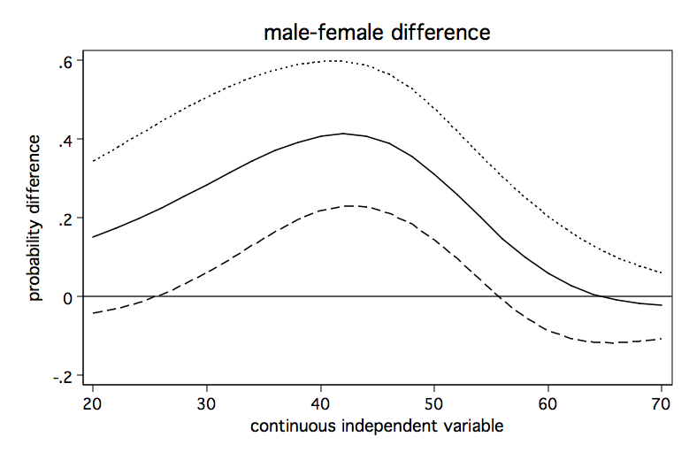
Next, we need to step through a bunch of different values for the of continuous predictor variable. The code fragment below will loop through 25 values of s between 20 and 70 while computing at differences in probability between f=0 and f=1. The code fragment will produce a graph of the difference in probability over the range of s.
forvalues x=20(2)70 {
  quietly prvalue, x(f=0 s=`x' fs=0)   save delta
  quietly prvalue, x(f=1 s=`x' fs=`x') diff delta
  matrix px  =(nullmat(px)    `x')
  matrix pdif=(nullmat(pdif)  pepred[6,2])
  matrix pup =(nullmat(pup)   peupper[6,2])
  matrix plo =(nullmat(plo)   pelower[6,2])
}
matrix P = px, pdif, plo, pup
matrix colnames P = xvar pdiff pdlo pdup
svmat P, names(col)
twoway line pdiff pdlo pdup xvar, yline(0) legend(off) name(pdiff, replace) sort ///
  xtitle(continuous independent variable) ytitle(probability difference) ///
  title(male-female difference)
Now, we will run the above code fragment and check out the graph.
The above graph shows how the male-female probability difference varies with changes in the value of s. It appears that the difference in probabilities for male and females is statistically significant between values of s of approximately 28 to 55 and is nonsignificant elsewhere.
So, that went fairly well but what if there was a covariate in the model? The model below includes the covariate cv1.
logit y f s fs cv1, nolog

Logistic regression                               Number of obs   =        200
                                                  LR chi2(4)      =     114.41
                                                  Prob > chi2     =     0.0000
Log likelihood = -74.587842                       Pseudo R2       =     0.4340

------------------------------------------------------------------------------
           y |      Coef.   Std. Err.      z    P>|z|     [95% Conf. Interval]
-------------+----------------------------------------------------------------
           f |   9.983662   3.052651     3.27   0.001     4.000576    15.96675
           s |   .1750686   .0470026     3.72   0.000     .0829452     .267192
          fs |  -.1595233   .0570345    -2.80   0.005    -.2713089   -.0477376
         cv1 |   .1877164   .0347886     5.40   0.000     .1195321    .2559008
       _cons |  -19.00557   3.371014    -5.64   0.000    -25.61264   -12.39851
------------------------------------------------------------------------------
As before, all of the coefficients are statistically significant.
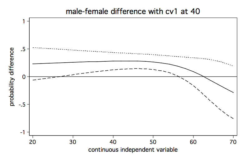
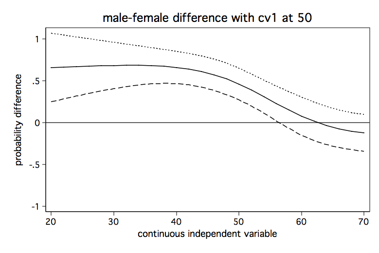
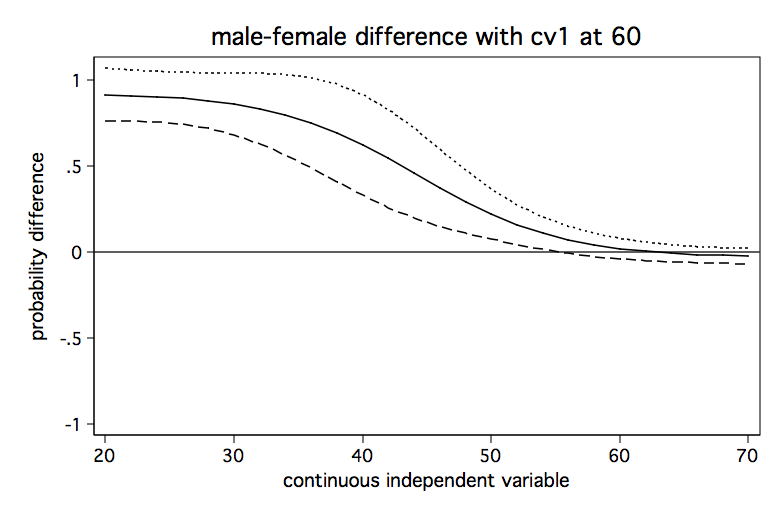
We will run the analysis pretty much as before except that we will do it three times holding the covariate at a different value each time. We begin holding the covariate at a low value of 40, then at a medium value of 50 and finally at a high value of 60. The code fragment below computes the predicted differences in probability for each of the three values of the covariate and produces a separate graph for each one.
/* hold cv1 at 40 */
forvalues x=20(2)70 {
  quietly prvalue, x(f=0 s=`x' fs=0   cv1=40) save delta
  quietly prvalue, x(f=1 s=`x' fs=`x' cv1=40) diff delta
  matrix px4  =(nullmat(px4)    `x')
  matrix pdif4=(nullmat(pdif4)  pepred[6,2])
  matrix pup4 =(nullmat(pup4)   peupper[6,2])
  matrix plo4 =(nullmat(plo4)   pelower[6,2])
 }
matrix P = px4, pdif4, plo4, pup4
matrix colnames P = xvar pdiff4 pdlo4 pdup4
svmat P, names(col)
twoway line pdiff4 pdlo4 pdup4 xvar, yline(0) legend(off) name(pdiff40, replace) sort ///
  ylabel(-1(.5)1) xtitle(continuous independent variable) ytitle(probability difference) ///
  title(male-female difference with cv1 at 40)

/* hold cv1 at 50 */
forvalues x=20(2)70 {
  quietly prvalue, x(f=0 s=`x' fs=0   cv1=50) save delta
  quietly prvalue, x(f=1 s=`x' fs=`x' cv1=50) diff delta
  matrix pdif5=(nullmat(pdif5)  pepred[6,2])
  matrix pup5 =(nullmat(pup5)   peupper[6,2])
  matrix plo5 =(nullmat(plo5)   pelower[6,2])
}
matrix P = pdif5, plo5, pup5
matrix colnames P = pdiff5 pdlo5 pdup5
svmat P, names(col)
twoway line pdiff5 pdlo5 pdup5 xvar, yline(0) legend(off) name(pdiff50, replace) sort ///
  ylabel(-1(.5)1) xtitle(continuous independent variable) ytitle(probability difference) ///
  title(male-female difference with cv1 at 50)

/* hold cv1 at 60 */
forvalues x=20(2)70 {
  quietly prvalue, x(f=0 s=`x' fs=0   cv1=60) save delta
  quietly prvalue, x(f=1 s=`x' fs=`x' cv1=60) diff delta
  matrix pdif6=(nullmat(pdif6)  pepred[6,2])
  matrix pup6 =(nullmat(pup6)   peupper[6,2])
  matrix plo6 =(nullmat(plo6)   pelower[6,2])
}
matrix P = pdif6, plo6, pup6
matrix colnames P = pdiff6 pdlo6 pdup6
svmat P, names(col)
twoway line pdiff6 pdlo6 pdup6 xvar, yline(0) legend(off) name(pdiff60, replace) sort ///
  ylabel(-1(.5)1) xtitle(continuous independent variable) ytitle(probability difference) ///
  title(male-female difference with cv1 at 60)
It seems clear from looking at the three graphs that the male-female difference in probability increases as cv1 increases except for high values of s. And, yes, I know the upper limit of the confidence interval exceeds one in some places but that is just an artifact of how the confidence intervals were created. We aren’t really trying to imply that the probability can ever exceed one.
Using predictnl
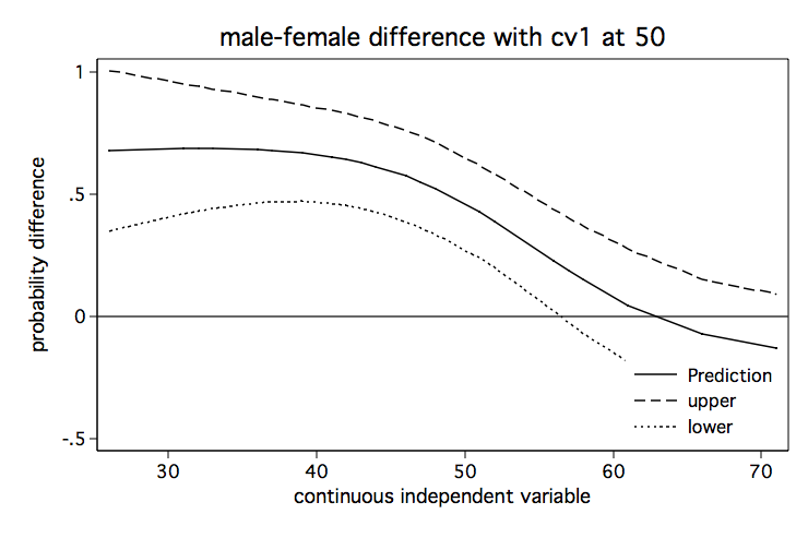
It is also possible to produce these graphs using the predictnl command after running the logistic regression. Below we show the code for producing the graph with the covariate, cv1 held at 50.
As the name suggests predictnl can calculate nonlinear predictions after any Stata estimation command and optionally calculates standard errors. We use predictnl to calculate the difference in probabilities. Here is how the parts of the prediction break out. The se() option creates a variable with the standard errors of the predicted values.
First, there is the probability for females.
exp(_b[_cons] + _b[s]*s + _b[cv1]*50+ _b[f] + _b[fs]*s)/(1+exp(_b[_cons] + _b[s]*s + _b[cv1]*50 + _b[f] + _b[fs]*s ))
Which is followed by the probability for males.
exp(_b[_cons] + _b[s]*s + _b[cv1]*50) /(1+exp(_b[_cons] + _b[s]*s + _b[cv1]*50))
Here is the complete code for computing the difference in probability and the generation of the graph.
predictnl diff_p = exp(_b[_cons] + _b[s]*s + _b[cv1]*50+ _b[f] + _b[fs]*s) ///
/(1+exp(_b[_cons] + _b[s]*s + _b[cv1]*50 + _b[f] + _b[fs]*s )) ///
- exp(_b[_cons] + _b[s]*s + _b[cv1]*50) /(1+exp(_b[_cons] + _b[s]*s + _b[cv1]*50)) ///
, se(diff_se)

gen upper = diff_p + diff_se*1.96
gen lower = diff_p - diff_se*1.96
sort s

twoway (line diff_p s) (line upper s) (line lower s), name(from_predictnl, replace) ///
       scheme(lean1) yline(0) legend(position(5) ring(0)) xtitle(continuous independent variable) ///
       ytitle(probability difference) title(male-female difference with cv1 at 50)
References
Long, J. S. 2006. Group comparisons and other issues in interpreting models for categorical
outcomes using Stata. Presentation at 5th North American Users Group Meeting. Boston,
Massachusetts.
Xu, J. and J.S. Long, 2005. Confidence intervals for predicted outcomes in regression models for
categorical outcomes. The Stata Journal 5: 537-559.

