The techniques and methods for this FAQ page were inspired Long (2006) and Hu & Long (2005).
Interactions in logistic regression models can be trickier than interactions in comparable OLS regression.
Many researchers are not comfortable interpreting the results in terms of the raw coefficients which are scaled in terms of log odds. The interpretation of interactions in log odds is done basically the same way as in OLS regression. However, many researchers prefer to interpret results in terms of probabilities. The shift from log odds to probabilities is a nonlinear transformation which means that the interactions are no longer a simple linear function of the predictors.
This FAQ page will try to help you to understand categorical by continuous interactions in logistic regression models both with and without covariates.
We will use an example dataset, logitcatcon, that has one binary predictor, f, which stands for female and one continuous predictor s. In addition, the model will include fs which is the f by s interaction. We will begin by loading the data and then running the logit model.
use https://stats.idre.ucla.edu/stat/data/logitcatcon, clear

logit y i.f##c.s, nolog

Logistic regression                               Number of obs   =        200
                                                  LR chi2(3)      =      71.01
                                                  Prob > chi2     =     0.0000
Log likelihood =  -96.28586                       Pseudo R2       =     0.2694

------------------------------------------------------------------------------
           y |      Coef.   Std. Err.      z    P>|z|     [95% Conf. Interval]
-------------+----------------------------------------------------------------
         1.f |   5.786811   2.302518     2.51   0.012     1.273959    10.29966
           s |   .1773383   .0364362     4.87   0.000     .1059248    .2487519
             |
       f#c.s |
          1  |  -.0895522   .0439158    -2.04   0.041    -.1756255   -.0034789
             |
       _cons |  -9.253801    1.94189    -4.77   0.000    -13.05983   -5.447767
------------------------------------------------------------------------------
As you can see all of the variables in the above model including the interaction term are statistically significant. If this were an OLS regression model we could do a very good job of understanding the interaction using just the coefficients in the model. The situation in logistic regression is more complicated because the value of the interaction effect changes depending upon the value of the continuous predictor variable. To begin to understand what is going on consider the Table 1 below.
Table 1: Predicted probabilities when s=40

     f=0     f=1    change     LB      UB
   .1034    .5111   .4077   .2182   .5972
Table 1 contains predicted probabilities, differences in predicted probabilities and the confidence interval of the difference in predicted probabilities while holding the continuous predictor at 40. The first value, .1034, is the predicted probability when f=0 (males), the .5111 when f=1 (females). The third value, .4077, is the difference in probabilities for males and females. The next two values are the 95% confidence interval on the difference in probabilities. If the confidence interval contains zero the difference would not be considered statistically significant. In our example, the confidence interval does not contain zero, thus, the difference in probabilities is statistically significant.
To get the values for Table 1 we will run margins twice. The second time we will use the dydx option to get the differences in probabilities. with the post option followed by the lincom command.
margins f, at(s=40)

Adjusted predictions                              Number of obs   =        200
Model VCE    : OIM

Expression   : Pr(y), predict()
at           : s               =          40

------------------------------------------------------------------------------
             |            Delta-method
             |     Margin   Std. Err.      z    P>|z|     [95% Conf. Interval]
-------------+----------------------------------------------------------------
           f |
          0  |   .1033756   .0500784     2.06   0.039     .0052238    .2015275
          1  |   .5111116   .0827069     6.18   0.000      .349009    .6732142
------------------------------------------------------------------------------

margins, dydx(f) at(s=40)

Conditional marginal effects                      Number of obs   =        200
Model VCE    : OIM

Expression   : Pr(y), predict()
dy/dx w.r.t. : 1.f

at           : s               =          40

------------------------------------------------------------------------------
             |            Delta-method
             |      dy/dx   Std. Err.      z    P>|z|     [95% Conf. Interval]
-------------+----------------------------------------------------------------
         1.f |    .407736   .0966865     4.22   0.000     .2182339     .597238
------------------------------------------------------------------------------
Note: dy/dx for factor levels is the discrete change from the base level.
Now that we know how to compute the difference in probabilities including the confidence intervals, we need to do this for a whole rang of values of s. The vsquish option just omits extra blank lines in the header.
margins, dydx(f) at(s=(20(2)70)) vsquish

Conditional marginal effects                      Number of obs   =        200
Model VCE    : OIM

Expression   : Pr(y), predict()
dy/dx w.r.t. : 1.f
1._at        : s               =          20
2._at        : s               =          22
3._at        : s               =          24
4._at        : s               =          26
5._at        : s               =          28
6._at        : s               =          30
7._at        : s               =          32
8._at        : s               =          34
9._at        : s               =          36
10._at       : s               =          38
11._at       : s               =          40
12._at       : s               =          42
13._at       : s               =          44
14._at       : s               =          46
15._at       : s               =          48
16._at       : s               =          50
17._at       : s               =          52
18._at       : s               =          54
19._at       : s               =          56
20._at       : s               =          58
21._at       : s               =          60
22._at       : s               =          62
23._at       : s               =          64
24._at       : s               =          66
25._at       : s               =          68
26._at       : s               =          70

------------------------------------------------------------------------------
             |            Delta-method
             |      dy/dx   Std. Err.      z    P>|z|     [95% Conf. Interval]
-------------+----------------------------------------------------------------
1.f          |
         _at |
          1  |   .1496878   .0987508     1.52   0.130    -.0438602    .3432358
          2  |   .1724472   .1043526     1.65   0.098    -.0320801    .3769745
          3  |   .1975119   .1089189     1.81   0.070    -.0159653    .4109891
          4  |   .2246979   .1121624     2.00   0.045     .0048636    .4445323
          5  |   .2536377   .1138457     2.23   0.026     .0305042    .4767711
          6  |   .2837288   .1138312     2.49   0.013     .0606236    .5068339
          7  |   .3140793   .1121391     2.80   0.005     .0942908    .5338679
          8  |   .3434564   .1090032     3.15   0.002     .1298141    .5570987
          9  |   .3702468    .104906     3.53   0.000     .1646348    .5758589
         10  |   .3924501    .100548     3.90   0.000     .1953797    .5895206
         11  |    .407736   .0966865     4.22   0.000     .2182339     .597238
         12  |   .4136138   .0938187     4.41   0.000     .2297325    .5974952
         13  |   .4077687   .0918544     4.44   0.000     .2277375       .5878
         14  |   .3885877   .0901232     4.31   0.000     .2119494     .565226
         15  |   .3558056   .0879135     4.05   0.000     .1834983     .528113
         16  |    .311046   .0851843     3.65   0.000     .1440878    .4780042
         17  |   .2579152   .0826761     3.12   0.002      .095873    .4199574
         18  |   .2014085   .0810274     2.49   0.013     .0425978    .3602193
         19  |    .146748   .0798151     1.84   0.066    -.0096868    .3031828
         20  |     .09816   .0778372     1.26   0.207    -.0543982    .2507182
         21  |   .0581376   .0741941     0.78   0.433    -.0872801    .2035553
         22  |   .0273908   .0688343     0.40   0.691    -.1075218    .1623035
         23  |   .0052927   .0623354     0.08   0.932    -.1168824    .1274678
         24  |  -.0095202   .0554486    -0.17   0.864    -.1181975    .0991571
         25  |  -.0186421   .0487849    -0.38   0.702    -.1142588    .0769746
         26  |  -.0235782    .042708    -0.55   0.581    -.1072843    .0601279
------------------------------------------------------------------------------
Note: dy/dx for factor levels is the discrete change from the base level.
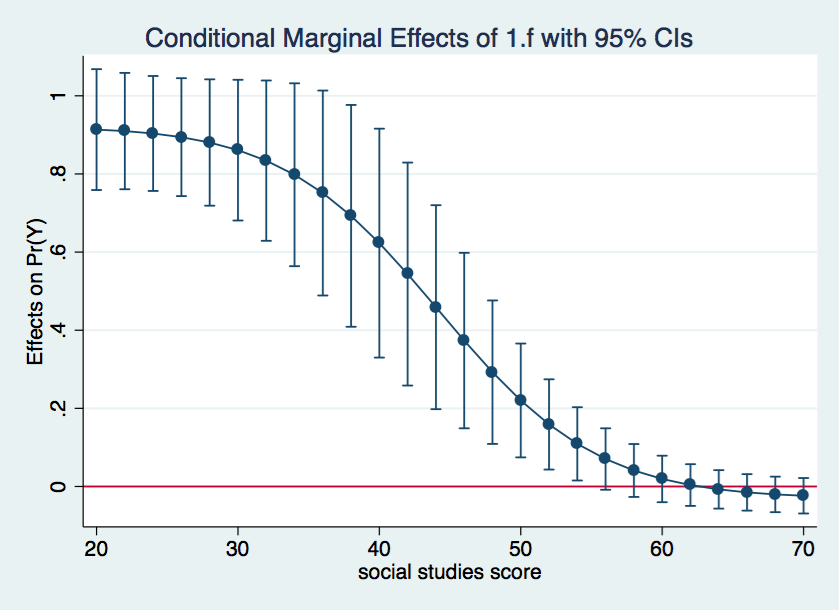
Now, we will graph the differences from the above table using the marginsplot command.
marginsplot, yline(0)
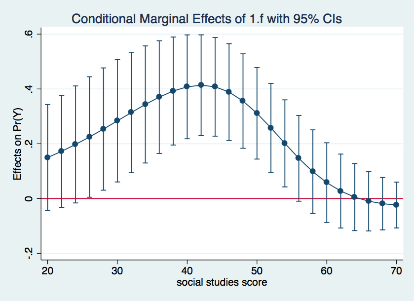
The above graph shows how the male-female probability difference varies with changes in the value of s. It appears that the difference in probabilities for male and females is statistically significant between values of s of approximately 28 to 55 and is nonsignificant elsewhere.
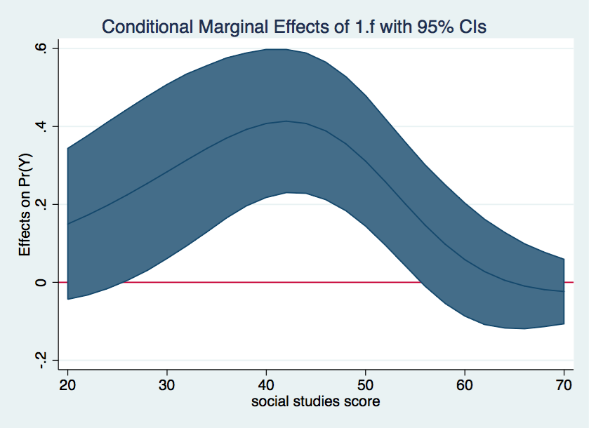
We can make the above graph a little more visually attractive by shading the
confidence intervals.
marginsplot, recast(line) recastci(rarea) yline(0)
Logit model with continuous covariate
So, that went fairly well but what if there was a covariate in the model? Adding covariates to a logit model can change the pattern of predicted probabilities even though the covariate does not interact with any of the primary research variables.
Our next model, shown below, includes the covariate cv1.
use https://stats.idre.ucla.edu/stat/data/logitcatcon, clear

logit y f##c.s cv1, nolog

Logistic regression                               Number of obs   =        200
                                                  LR chi2(4)      =     114.41
                                                  Prob > chi2     =     0.0000
Log likelihood = -74.587842                       Pseudo R2       =     0.4340

------------------------------------------------------------------------------
           y |      Coef.   Std. Err.      z    P>|z|     [95% Conf. Interval]
-------------+----------------------------------------------------------------
         1.f |   9.983662    3.05269     3.27   0.001       4.0005    15.96682
           s |   .1750686   .0470033     3.72   0.000     .0829438    .2671933
             |
       f#c.s |
          1  |  -.1595233   .0570352    -2.80   0.005    -.2713103   -.0477363
             |
         cv1 |   .1877164   .0347888     5.40   0.000     .1195316    .2559013
       _cons |  -19.00557   3.371064    -5.64   0.000    -25.61273   -12.39841
------------------------------------------------------------------------------
As before, all of the coefficients are statistically significant.
We will run the analysis pretty much as before except that we will do it three times holding the covariate at a different value each time. We begin holding the covariate at a low value of 40, then at a medium value of 50 and finally at a high value of 60. The commands compute the predicted differences in probability for each of the three values of the covariate and produces a separate graph for each one.
margins, dydx(f) at(s=(20(2)70) cv1=40) noatlegend
Conditional marginal effects Number of obs = 200
Model VCE : OIM
Expression : Pr(y), predict()
dy/dx w.r.t. : 1.f
------------------------------------------------------------------------------
| Delta-method
| dy/dx Std. Err. z P>|z| [95% Conf. Interval]
-------------+----------------------------------------------------------------
1.f |
_at |
1 | .2307214 .150045 1.54 0.124 -.0633615 .5248042
2 | .2361502 .1429905 1.65 0.099 -.044106 .5164064
3 | .2416119 .1357653 1.78 0.075 -.0244832 .5077069
4 | .2470812 .1284098 1.92 0.054 -.0045973 .4987597
5 | .2525225 .1209752 2.09 0.037 .0154154 .4896296
6 | .2578855 .1135271 2.27 0.023 .0353765 .4803946
7 | .2630995 .1061484 2.48 0.013 .0550525 .4711464
8 | .2680645 .0989437 2.71 0.007 .0741384 .4619905
9 | .2726404 .0920437 2.96 0.003 .0922382 .4530427
10 | .2766309 .0856081 3.23 0.001 .1088422 .4444197
11 | .2797622 .0798258 3.50 0.000 .1233066 .4362179
12 | .2816551 .0749086 3.76 0.000 .134837 .4284732
13 | .2817895 .0710764 3.96 0.000 .1424822 .4210967
14 | .2794619 .0685404 4.08 0.000 .1451252 .4137986
15 | .2737404 .0675055 4.06 0.000 .141432 .4060488
16 | .2634265 .0682395 3.86 0.000 .1296795 .3971735
17 | .247046 .0712461 3.47 0.001 .1074062 .3866859
18 | .2229048 .0774966 2.88 0.004 .0710142 .3747954
19 | .1892608 .0884614 2.14 0.032 .0158797 .3626418
20 | .1446609 .1055661 1.37 0.171 -.0622448 .3515666
21 | .08845 .1291224 0.69 0.493 -.1646253 .3415252
22 | .0213483 .1574555 0.14 0.892 -.2872588 .3299553
23 | -.0541486 .1869312 -0.29 0.772 -.420527 .3122298
24 | -.1338606 .2130623 -0.63 0.530 -.5514551 .2837339
25 | -.212654 .2323119 -0.92 0.360 -.6679769 .242669
26 | -.2855934 .2436296 -1.17 0.241 -.7630986 .1919118
------------------------------------------------------------------------------
Note: dy/dx for factor levels is the discrete change from the base level.
marginsplot, yline(0)
 margins, dydx(f) at(s=(20(2)70) cv1=50) noatlegend
Conditional marginal effects Number of obs = 200
Model VCE : OIM
Expression : Pr(y), predict()
dy/dx w.r.t. : 1.f
------------------------------------------------------------------------------
| Delta-method
| dy/dx Std. Err. z P>|z| [95% Conf. Interval]
-------------+----------------------------------------------------------------
1.f |
_at |
1 | .6603841 .2089015 3.16 0.002 .2509446 1.069824
2 | .6663811 .1945798 3.42 0.001 .2850117 1.047751
3 | .6719235 .1806131 3.72 0.000 .3179283 1.025919
4 | .6768518 .167067 4.05 0.000 .3494065 1.004297
5 | .6809438 .1540312 4.42 0.000 .3790483 .9828394
6 | .6838906 .1416328 4.83 0.000 .4062954 .9614859
7 | .6852664 .1300559 5.27 0.000 .4303616 .9401712
8 | .6844899 .1195626 5.72 0.000 .4501515 .9188282
9 | .6807804 .1105069 6.16 0.000 .4641908 .89737
10 | .6731136 .1033086 6.52 0.000 .4706324 .8755948
11 | .6601906 .0983425 6.71 0.000 .4674428 .8529385
12 | .6404474 .0957213 6.69 0.000 .4528371 .8280577
13 | .612146 .0950685 6.44 0.000 .4258151 .7984768
14 | .5736015 .0955153 6.01 0.000 .386395 .760808
15 | .5235847 .0961089 5.45 0.000 .3352148 .7119546
16 | .4618751 .0965359 4.78 0.000 .2726681 .651082
17 | .3898094 .0976254 3.99 0.000 .1984672 .5811516
18 | .310538 .1007595 3.08 0.002 .113053 .5080229
19 | .2287029 .1061749 2.15 0.031 .0206039 .436802
20 | .1495094 .1121609 1.33 0.183 -.0703219 .3693407
21 | .0775412 .1164177 0.67 0.505 -.1506333 .3057156
22 | .0158576 .1177948 0.13 0.893 -.215016 .2467312
23 | -.0342943 .1167353 -0.29 0.769 -.2630913 .1945027
24 | -.0732007 .1146282 -0.64 0.523 -.2978678 .1514664
25 | -.102126 .1129167 -0.90 0.366 -.3234388 .1191867
26 | -.1227649 .1125169 -1.09 0.275 -.3432941 .0977642
------------------------------------------------------------------------------
Note: dy/dx for factor levels is the discrete change from the base level.
marginsplot, yline(0)
margins, dydx(f) at(s=(20(2)70) cv1=50) noatlegend
Conditional marginal effects Number of obs = 200
Model VCE : OIM
Expression : Pr(y), predict()
dy/dx w.r.t. : 1.f
------------------------------------------------------------------------------
| Delta-method
| dy/dx Std. Err. z P>|z| [95% Conf. Interval]
-------------+----------------------------------------------------------------
1.f |
_at |
1 | .6603841 .2089015 3.16 0.002 .2509446 1.069824
2 | .6663811 .1945798 3.42 0.001 .2850117 1.047751
3 | .6719235 .1806131 3.72 0.000 .3179283 1.025919
4 | .6768518 .167067 4.05 0.000 .3494065 1.004297
5 | .6809438 .1540312 4.42 0.000 .3790483 .9828394
6 | .6838906 .1416328 4.83 0.000 .4062954 .9614859
7 | .6852664 .1300559 5.27 0.000 .4303616 .9401712
8 | .6844899 .1195626 5.72 0.000 .4501515 .9188282
9 | .6807804 .1105069 6.16 0.000 .4641908 .89737
10 | .6731136 .1033086 6.52 0.000 .4706324 .8755948
11 | .6601906 .0983425 6.71 0.000 .4674428 .8529385
12 | .6404474 .0957213 6.69 0.000 .4528371 .8280577
13 | .612146 .0950685 6.44 0.000 .4258151 .7984768
14 | .5736015 .0955153 6.01 0.000 .386395 .760808
15 | .5235847 .0961089 5.45 0.000 .3352148 .7119546
16 | .4618751 .0965359 4.78 0.000 .2726681 .651082
17 | .3898094 .0976254 3.99 0.000 .1984672 .5811516
18 | .310538 .1007595 3.08 0.002 .113053 .5080229
19 | .2287029 .1061749 2.15 0.031 .0206039 .436802
20 | .1495094 .1121609 1.33 0.183 -.0703219 .3693407
21 | .0775412 .1164177 0.67 0.505 -.1506333 .3057156
22 | .0158576 .1177948 0.13 0.893 -.215016 .2467312
23 | -.0342943 .1167353 -0.29 0.769 -.2630913 .1945027
24 | -.0732007 .1146282 -0.64 0.523 -.2978678 .1514664
25 | -.102126 .1129167 -0.90 0.366 -.3234388 .1191867
26 | -.1227649 .1125169 -1.09 0.275 -.3432941 .0977642
------------------------------------------------------------------------------
Note: dy/dx for factor levels is the discrete change from the base level.
marginsplot, yline(0)
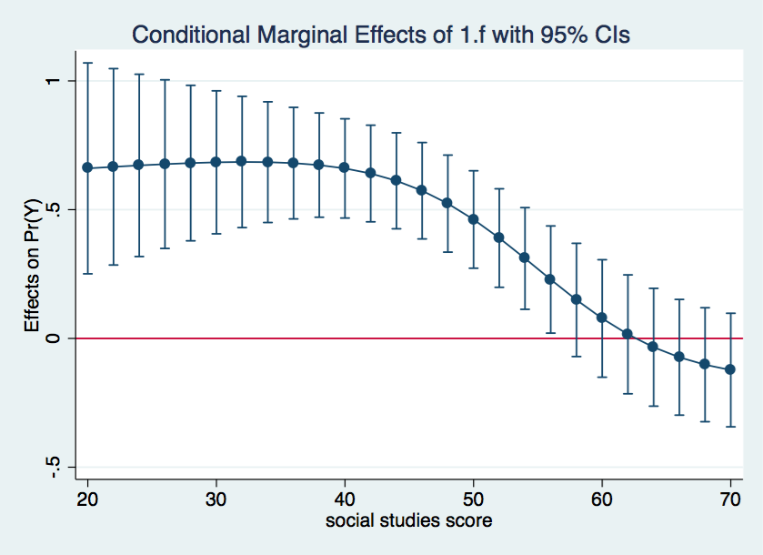 margins, dydx(f) at(s=(20(2)70) cv1=60) noatlegend
Conditional marginal effects Number of obs = 200
Model VCE : OIM
Expression : Pr(y), predict()
dy/dx w.r.t. : 1.f
------------------------------------------------------------------------------
| Delta-method
| dy/dx Std. Err. z P>|z| [95% Conf. Interval]
-------------+----------------------------------------------------------------
1.f |
_at |
1 | .9135206 .0789176 11.58 0.000 .7588449 1.068196
2 | .9097497 .0759899 11.97 0.000 .7608121 1.058687
3 | .903598 .0750691 12.04 0.000 .7564654 1.050731
4 | .8942046 .0769878 11.61 0.000 .7433112 1.045098
5 | .8804504 .0825006 10.67 0.000 .7187522 1.042149
6 | .860939 .0918979 9.37 0.000 .6808225 1.041056
7 | .8340294 .1046826 7.97 0.000 .6288553 1.039203
8 | .79797 .1194328 6.68 0.000 .5638859 1.032054
9 | .7511866 .1338225 5.61 0.000 .4888992 1.013474
10 | .6927478 .1448523 4.78 0.000 .4088424 .9766531
11 | .6229422 .1494681 4.17 0.000 .3299901 .9158944
12 | .5437595 .1455949 3.73 0.000 .2583987 .8291202
13 | .4589623 .1331889 3.45 0.001 .1979168 .7200079
14 | .3735294 .1145842 3.26 0.001 .1489486 .5981102
15 | .2925756 .0936809 3.12 0.002 .1089644 .4761868
16 | .2202105 .0743402 2.96 0.003 .0745063 .3659147
17 | .1588388 .0589333 2.70 0.007 .0433317 .274346
18 | .1091008 .0478486 2.28 0.023 .0153193 .2028823
19 | .0702892 .0401238 1.75 0.080 -.008352 .1489304
20 | .0409283 .0345573 1.18 0.236 -.0268028 .1086594
21 | .0192749 .0303776 0.63 0.526 -.0402642 .0788139
22 | .0036462 .0272628 0.13 0.894 -.0497878 .0570803
23 | -.0074154 .0251015 -0.30 0.768 -.0566134 .0417827
24 | -.0150913 .0238003 -0.63 0.526 -.061739 .0315564
25 | -.0202982 .0232115 -0.87 0.382 -.0657919 .0251955
26 | -.0237264 .02315 -1.02 0.305 -.0690996 .0216469
------------------------------------------------------------------------------
Note: dy/dx for factor levels is the discrete change from the base level.
marginsplot, yline(0)
margins, dydx(f) at(s=(20(2)70) cv1=60) noatlegend
Conditional marginal effects Number of obs = 200
Model VCE : OIM
Expression : Pr(y), predict()
dy/dx w.r.t. : 1.f
------------------------------------------------------------------------------
| Delta-method
| dy/dx Std. Err. z P>|z| [95% Conf. Interval]
-------------+----------------------------------------------------------------
1.f |
_at |
1 | .9135206 .0789176 11.58 0.000 .7588449 1.068196
2 | .9097497 .0759899 11.97 0.000 .7608121 1.058687
3 | .903598 .0750691 12.04 0.000 .7564654 1.050731
4 | .8942046 .0769878 11.61 0.000 .7433112 1.045098
5 | .8804504 .0825006 10.67 0.000 .7187522 1.042149
6 | .860939 .0918979 9.37 0.000 .6808225 1.041056
7 | .8340294 .1046826 7.97 0.000 .6288553 1.039203
8 | .79797 .1194328 6.68 0.000 .5638859 1.032054
9 | .7511866 .1338225 5.61 0.000 .4888992 1.013474
10 | .6927478 .1448523 4.78 0.000 .4088424 .9766531
11 | .6229422 .1494681 4.17 0.000 .3299901 .9158944
12 | .5437595 .1455949 3.73 0.000 .2583987 .8291202
13 | .4589623 .1331889 3.45 0.001 .1979168 .7200079
14 | .3735294 .1145842 3.26 0.001 .1489486 .5981102
15 | .2925756 .0936809 3.12 0.002 .1089644 .4761868
16 | .2202105 .0743402 2.96 0.003 .0745063 .3659147
17 | .1588388 .0589333 2.70 0.007 .0433317 .274346
18 | .1091008 .0478486 2.28 0.023 .0153193 .2028823
19 | .0702892 .0401238 1.75 0.080 -.008352 .1489304
20 | .0409283 .0345573 1.18 0.236 -.0268028 .1086594
21 | .0192749 .0303776 0.63 0.526 -.0402642 .0788139
22 | .0036462 .0272628 0.13 0.894 -.0497878 .0570803
23 | -.0074154 .0251015 -0.30 0.768 -.0566134 .0417827
24 | -.0150913 .0238003 -0.63 0.526 -.061739 .0315564
25 | -.0202982 .0232115 -0.87 0.382 -.0657919 .0251955
26 | -.0237264 .02315 -1.02 0.305 -.0690996 .0216469
------------------------------------------------------------------------------
Note: dy/dx for factor levels is the discrete change from the base level.
marginsplot, yline(0)
That went well, so let’s try to combine all three graphs into one. We will rerun the margins command using the quietly option to suppress the output which we have seen above.
quietly margins, dydx(f) at(s=(20(2)70) cv1=(40 50 60))

marginsplot, yline(0)
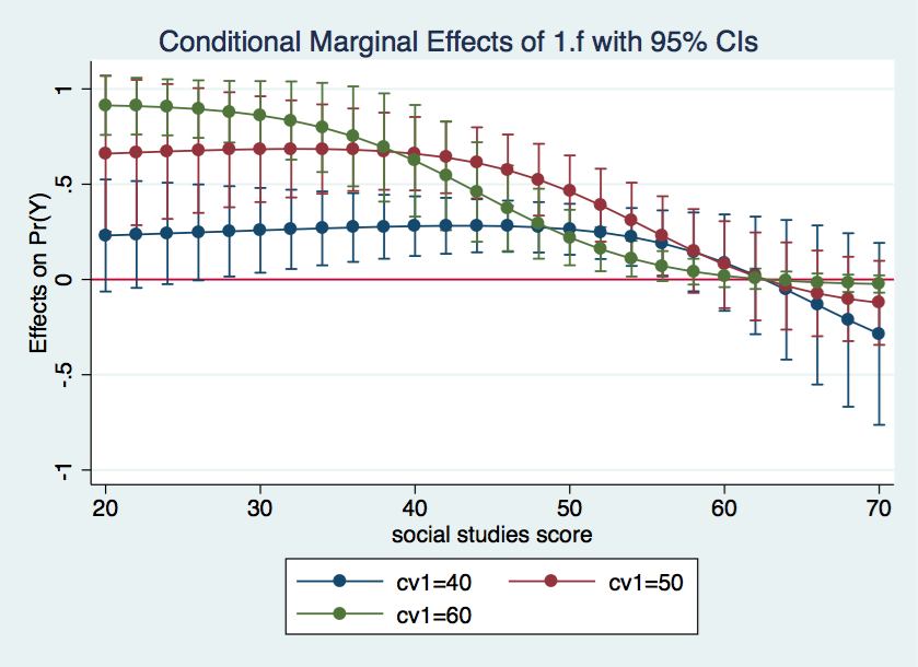
It seems clear from looking at the three graphs that the male-female difference in probability increases as cv1 increases except for high values of s. And, yes, I know the upper limit of the confidence interval exceeds one in some places but that is just an artifact of how the confidence intervals were created. We aren’t really trying to imply that the probability can ever exceed one.
One final graph with shaded confidence intervals and we’re done.
marginsplot, recast(line) recastci(rarea) yline(0)
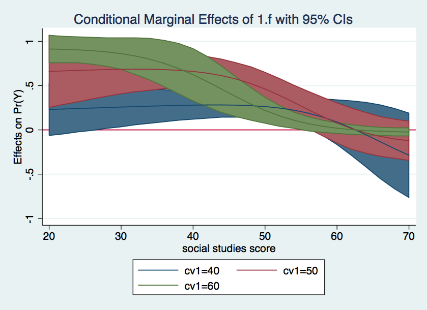
Awesome graph!
References
Long, J. S. 2006. Group comparisons and other issues in interpreting models for categorical outcomes using Stata. Presentation at 5th North American Users Group Meeting. Boston, Massachusetts. Xu, J. and J.S. Long, 2005. Confidence intervals for predicted outcomes in regression models for categorical outcomes. The Stata Journal 5: 537-559.