
Interpreting interactions in ologit is similar interpreting interactions in
logit with the complication of multiple equations. We will demonstrate a
categorical by continuous interaction using the hsbdemo dataset. We will
use ses as the response variable. I know that its not a great choice as an
outcome but it is ordinal with values 1, 2 and 3.
use https://stats.idre.ucla.edu/stat/data/hsbdemo, clear

ologit ses i.female##c.read science

Iteration 0:   log likelihood = -210.58254
Iteration 1:   log likelihood = -197.30785
Iteration 2:   log likelihood = -197.14337
Iteration 3:   log likelihood = -197.14305
Iteration 4:   log likelihood = -197.14305

Ordered logistic regression                     Number of obs     =        200
                                                LR chi2(4)        =      26.88
                                                Prob > chi2       =     0.0000
Log likelihood = -197.14305                     Pseudo R2         =     0.0638

-------------------------------------------------------------------------------
          ses |      Coef.   Std. Err.      z    P>|z|     [95% Conf. Interval]
--------------+----------------------------------------------------------------
       female |
      female  |  -2.827935    1.44449    -1.96   0.050    -5.659084    .0032144
         read |   .0134508   .0225948     0.60   0.552    -.0308341    .0577357
              |
female#c.read |
      female  |   .0474638   .0272074     1.74   0.081    -.0058617    .1007894
              |
      science |   .0352044   .0187329     1.88   0.060    -.0015115    .0719202
--------------+----------------------------------------------------------------
        /cut1 |   1.014755   1.073606                     -1.089474    3.118984
        /cut2 |   3.323198   1.102349                      1.162633    5.483762
-------------------------------------------------------------------------------
The interaction term is statistically significant.
We can use the margins command to get the expected probability that the outcome
will be a one for males and females for various values of read.
We have to do this for each of the values of the response variable. After obtaining
the predicted probabilities we will plot these using marginsplot.
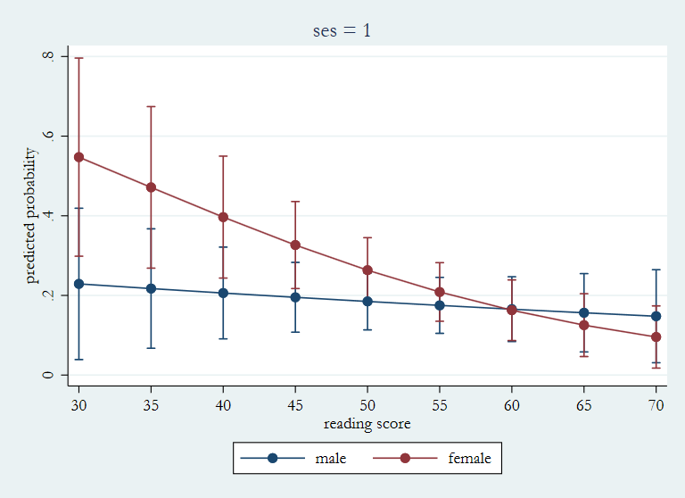
Let’s begin with ses = 1.
margins female, at(read=(30(5)70)) atmeans noatlegend predict(outcome(1))

Adjusted predictions                            Number of obs     =        200
Model VCE    : OIM

Expression   : Pr(ses==1), predict(outcome(1))

------------------------------------------------------------------------------
             |            Delta-method
             |     Margin   Std. Err.      z    P>|z|     [95% Conf. Interval]
-------------+----------------------------------------------------------------
  _at#female |
     1#male  |   .2289736   .0969437     2.36   0.018     .0389675    .4189797
   1#female  |   .5473337   .1269408     4.31   0.000     .2985343    .7961331
     2#male  |   .2173171   .0765414     2.84   0.005     .0672987    .3673355
   2#female  |   .4713639   .1035006     4.55   0.000     .2685065    .6742213
     3#male  |   .2060954   .0587678     3.51   0.000     .0909126    .3212782
   3#female  |   .3966979   .0780863     5.08   0.000     .2436515    .5497442
     4#male  |   .1953085   .0447382     4.37   0.000     .1076233    .2829938
   4#female  |   .3265531   .0557585     5.86   0.000     .2172686    .4358377
     5#male  |   .1849547   .0364871     5.07   0.000     .1134413    .2564682
   5#female  |   .2633964   .0416219     6.33   0.000      .181819    .3449737
     6#male  |   .1750304   .0358565     4.88   0.000      .104753    .2453078
   6#female  |   .2086696   .0375323     5.56   0.000     .1351077    .2822316
     7#male  |   .1655305    .041501     3.99   0.000       .08419     .246871
   7#female  |   .1628005   .0388408     4.19   0.000      .086674    .2389271
     8#male  |   .1564484   .0501496     3.12   0.002     .0581569    .2547399
   8#female  |   .1254162   .0402511     3.12   0.002     .0465256    .2043069
     9#male  |   .1477763   .0596128     2.48   0.013     .0309374    .2646152
   9#female  |   .0956359   .0398247     2.40   0.016      .017581    .1736909
------------------------------------------------------------------------------


marginsplot, x(read) title(ses = 1) ytitle(predicted probability) ///
  ylabel(0(.2).8) name(ses1, replace)
That worked pretty well, so let’s repeat it for ses = 2 and 3.
margins female, at(read=(30(5)70)) atmeans noatlegend predict(outcome(2))
Adjusted predictions Number of obs = 200
Model VCE : OIM
Expression : Pr(ses==2), predict(outcome(2))
------------------------------------------------------------------------------
| Delta-method
| Margin Std. Err. z P>|z| [95% Conf. Interval]
-------------+----------------------------------------------------------------
_at#female |
1#male | .5202219 .0387564 13.42 0.000 .4442608 .596183
1#female | .376692 .0928976 4.05 0.000 .1946161 .558768
2#male | .5190308 .0394899 13.14 0.000 .441632 .5964295
2#female | .4283249 .0705791 6.07 0.000 .2899924 .5666575
3#male | .51699 .0397363 13.01 0.000 .4391082 .5948717
3#female | .4719663 .0511282 9.23 0.000 .3717569 .5721757
4#male | .5141104 .0393479 13.07 0.000 .43699 .5912309
4#female | .5033055 .0406159 12.39 0.000 .4236998 .5829112
5#male | .5104075 .0387839 13.16 0.000 .4343924 .5864226
5#female | .5190623 .038373 13.53 0.000 .4438525 .5942721
6#male | .505901 .039099 12.94 0.000 .4292683 .5825336
6#female | .5175406 .0385338 13.43 0.000 .4420157 .5930654
7#male | .5006147 .0417421 11.99 0.000 .4188016 .5824277
7#female | .4989053 .0418322 11.93 0.000 .4169157 .580895
8#male | .4945765 .0479154 10.32 0.000 .4006639 .588489
8#female | .4651562 .0540699 8.60 0.000 .3591811 .5711312
9#male | .487818 .0579665 8.42 0.000 .3742058 .6014303
9#female | .4197988 .0744192 5.64 0.000 .27394 .5656577
------------------------------------------------------------------------------
marginsplot, x(read) title(ses = 2) ytitle(predicted probability) ///
ylabel(0(.2).8) name(ses2, replace)
 margins female, at(read=(30(5)70)) atmeans noatlegend predict(outcome(3))
Adjusted predictions Number of obs = 200
Model VCE : OIM
Expression : Pr(ses==3), predict(outcome(3))
------------------------------------------------------------------------------
| Delta-method
| Margin Std. Err. z P>|z| [95% Conf. Interval]
-------------+----------------------------------------------------------------
_at#female |
1#male | .2508045 .1028448 2.44 0.015 .0492325 .4523765
1#female | .0759742 .0381832 1.99 0.047 .0011366 .1508118
2#male | .2636521 .0865142 3.05 0.002 .0940873 .433217
2#female | .1003111 .0401995 2.50 0.013 .0215215 .1791007
3#male | .2769147 .0702594 3.94 0.000 .1392087 .4146206
3#female | .1313358 .0403181 3.26 0.001 .0523138 .2103578
4#male | .290581 .0557681 5.21 0.000 .1812776 .3998845
4#female | .1701414 .0387391 4.39 0.000 .0942141 .2460687
5#male | .3046377 .0467844 6.51 0.000 .2129421 .3963334
5#female | .2175413 .0378984 5.74 0.000 .1432618 .2918209
6#male | .3190686 .0485295 6.57 0.000 .2239524 .4141848
6#female | .2737898 .043457 6.30 0.000 .1886156 .358964
7#male | .3338548 .0615257 5.43 0.000 .2132666 .454443
7#female | .3382941 .0591724 5.72 0.000 .2223183 .4542699
8#male | .3489751 .0815056 4.28 0.000 .1892272 .5087231
8#female | .4094276 .0823118 4.97 0.000 .2480995 .5707557
9#male | .3644056 .1052248 3.46 0.001 .1581689 .5706424
9#female | .4845652 .1076582 4.50 0.000 .273559 .6955714
------------------------------------------------------------------------------
marginsplot, x(read) title(ses = 3) ytitle(predicted probability) ///
ylabel(0(.2).8) name(ses3, replace)
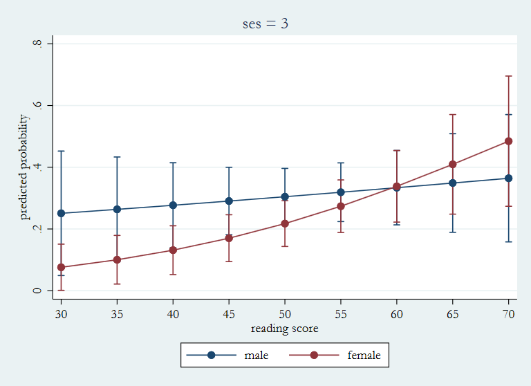
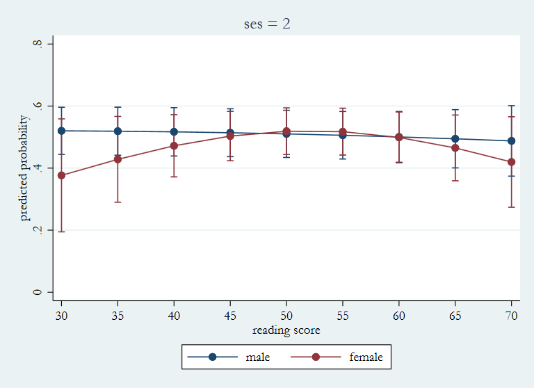
As you can see the patterns of predicted probabilities for the three vales of ses
are very different. The pattern trends down toward the right for ses = 1 with females having
the higher probabilities. For ses = 3 the trend is up toward the right with males having
the higher probabilities. While for ses = 2 the lines of the predicted probabilities
cross over one another.
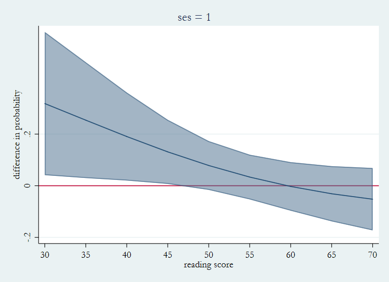
Another way to look at this is to look at the difference in predicted probabilities between males and females
for each value of read by using the dydx option.
margins, dydx(female) at(read=(30(5)70)) atmeans noatlegend predict(outcome(1))
Conditional marginal effects Number of obs = 200
Model VCE : OIM
Expression : Pr(ses==1), predict(outcome(1))
dy/dx w.r.t. : 1.female
------------------------------------------------------------------------------
| Delta-method
| dy/dx Std. Err. z P>|z| [95% Conf. Interval]
-------------+----------------------------------------------------------------
0.female | (base outcome)
-------------+----------------------------------------------------------------
1.female |
_at |
1 | .3183601 .1414102 2.25 0.024 .0412011 .5955191
2 | .2540468 .1143787 2.22 0.026 .0298686 .478225
3 | .1906025 .0869259 2.19 0.028 .0202309 .360974
4 | .1312446 .0632798 2.07 0.038 .0072184 .2552708
5 | .0784416 .0481498 1.63 0.103 -.0159302 .1728134
6 | .0336392 .0441156 0.76 0.446 -.0528258 .1201042
7 | -.00273 .04791 -0.06 0.955 -.0966318 .0911719
8 | -.0310321 .0545057 -0.57 0.569 -.1378613 .075797
9 | -.0521404 .0615919 -0.85 0.397 -.1728584 .0685776
------------------------------------------------------------------------------
Note: dy/dx for factor levels is the discrete change from the base level.
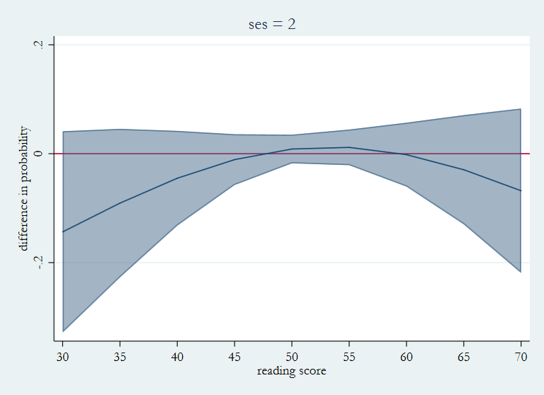
marginsplot, x(read) recast(line) recastci(rarea) ciopt(color(%50)) ///
title(ses = 1) ytitle(difference in probability) ///
ylabel(-.2(.2).2) yline(0) name(dses1, replace)
 margins, dydx(female) at(read=(30(5)70)) atmeans noatlegend predict(outcome(2))
Conditional marginal effects Number of obs = 200
Model VCE : OIM
Expression : Pr(ses==2), predict(outcome(2))
dy/dx w.r.t. : 1.female
------------------------------------------------------------------------------
| Delta-method
| dy/dx Std. Err. z P>|z| [95% Conf. Interval]
-------------+----------------------------------------------------------------
0.female | (base outcome)
-------------+----------------------------------------------------------------
1.female |
_at |
1 | -.1435299 .0942982 -1.52 0.128 -.3283509 .0412912
2 | -.0907058 .0695967 -1.30 0.192 -.2271128 .0457011
3 | -.0450237 .0443645 -1.01 0.310 -.1319764 .0419291
4 | -.0108049 .0238153 -0.45 0.650 -.0574821 .0358723
5 | .0086548 .0134412 0.64 0.520 -.0176895 .034999
6 | .0116396 .0166958 0.70 0.486 -.0210835 .0443627
7 | -.0017093 .0299499 -0.06 0.954 -.0604101 .0569915
8 | -.0294203 .0511755 -0.57 0.565 -.1297226 .0708819
9 | -.0680192 .0771124 -0.88 0.378 -.2191566 .0831183
------------------------------------------------------------------------------
Note: dy/dx for factor levels is the discrete change from the base level.
marginsplot, x(read) recast(line) recastci(rarea) ciopt(color(%50)) ///
title(ses = 2) ytitle(difference in probability) ///
ylabel(-.2(.2).2) yline(0) name(dses2, replace)
 margins, dydx(female) at(read=(30(5)70)) atmeans noatlegend predict(outcome(3))
Conditional marginal effects Number of obs = 200
Model VCE : OIM
Expression : Pr(ses==3), predict(outcome(3))
dy/dx w.r.t. : 1.female
------------------------------------------------------------------------------
| Delta-method
| dy/dx Std. Err. z P>|z| [95% Conf. Interval]
-------------+----------------------------------------------------------------
0.female | (base outcome)
-------------+----------------------------------------------------------------
1.female |
_at |
1 | -.1748303 .0997897 -1.75 0.080 -.3704146 .020754
2 | -.163341 .0852868 -1.92 0.055 -.3305 .003818
3 | -.1455788 .0714934 -2.04 0.042 -.2857034 -.0054543
4 | -.1204397 .0598967 -2.01 0.044 -.2378351 -.0030442
5 | -.0870964 .0541467 -1.61 0.108 -.1932219 .0190291
6 | -.0452788 .0597056 -0.76 0.448 -.1622995 .071742
7 | .0044393 .0778516 0.06 0.955 -.148147 .1570255
8 | .0604525 .104374 0.58 0.562 -.1441169 .2650218
9 | .1201596 .1343573 0.89 0.371 -.143176 .3834951
------------------------------------------------------------------------------
Note: dy/dx for factor levels is the discrete change from the base level.
marginsplot, x(read) recast(line) recastci(rarea) ciopt(color(%50)) ///
title(ses = 3) ytitle(difference in probability) ///
ylabel(-.2(.2).2) yline(0) name(dses3, replace)
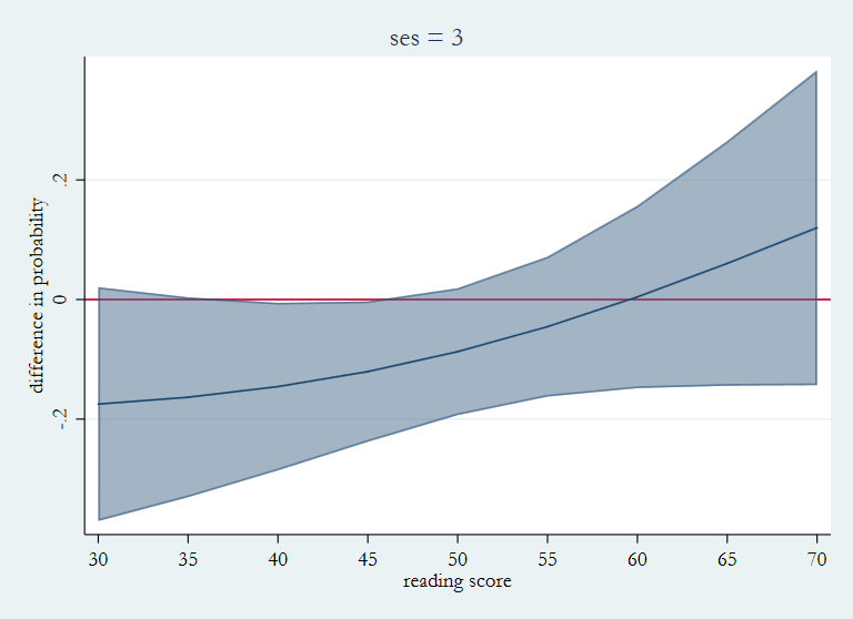
This time the difference in the three plots is more subtle. For ses = 1 all of the
differences are positive and grow smaller as you move from left to right. For ses
= 3 the differences are all negative and grow slightly large as read increases.
For ses = 2 the difference in probability start off negative becoming positive
around read = 50.