Continuous by continuous interactions in OLS regression can be tricky. Continuous by continuous interactions in logistic regression can be downright nasty. However, with the assistance of the margins command (introduced in Stata 11) and the margins command (introduced in Stata 12), we will be able to tame those continuous by continuous logistic interactions.
Most researchers are not comfortable interpreting logistic regression results in terms of the raw coefficients which are scaled in terms of log odds. Interpreting logistic interaction in terms of odds ratios is not much easier. Many researchers prefer to interpret logistic interaction results in terms of probabilities. The shift from log odds to probabilities is a nonlinear transformation which means that the interactions are no longer a simple linear function of the predictors. This FAQ page will try to help you to understand continuous by continuous interactions in logistic regression models both with and without covariates.
We will use an example dataset, logitconcon, that has two continuous predictors, r and m and a binary response variable y. It also has a continuous covariate, cv1, which we will use in a later model. We will begin by loading the data and running a logistic regression model with an interaction term.
use https://stats.idre.ucla.edu/stat/data/logitconcon, clear

logit y c.r##c.m, nolog

Logistic regression                               Number of obs   =        200
                                                  LR chi2(3)      =      65.47
                                                  Prob > chi2     =     0.0000
Log likelihood = -78.621746                       Pseudo R2       =     0.2940

------------------------------------------------------------------------------
           y |      Coef.   Std. Err.      z    P>|z|     [95% Conf. Interval]
-------------+----------------------------------------------------------------
           r |   .4407548   .1934232     2.28   0.023     .0616522    .8198573
           m |   .5069182   .1984649     2.55   0.011     .1179343    .8959022
             |
     c.r#c.m |  -.0066735   .0032877    -2.03   0.042    -.0131173   -.0002298
             |
       _cons |   -32.9762   11.49797    -2.87   0.004    -55.51182   -10.44059
------------------------------------------------------------------------------
As you can see all of the variables in the above model including the interaction term are statistically significant. What we will want to do is to see what a one unit change in r has on the probability when m is held constant at different values. We can do this easily using the margins command. Here is what the command looks like holding m constant for every five values between 30 and 70. We will use the post option so that we can use parmest (search parmest) to save the estimates to memory as data.
margins, dydx(r) at(m=(30(5)70)) vsquish

Average marginal effects                          Number of obs   =        200
Model VCE    : OIM

Expression   : Pr(y), predict()
dy/dx w.r.t. : r
1._at        : m               =          30
2._at        : m               =          35
3._at        : m               =          40
4._at        : m               =          45
5._at        : m               =          50
6._at        : m               =          55
7._at        : m               =          60
8._at        : m               =          65
9._at        : m               =          70

------------------------------------------------------------------------------
             |            Delta-method
             |      dy/dx   Std. Err.      z    P>|z|     [95% Conf. Interval]
-------------+----------------------------------------------------------------
r            |
         _at |
          1  |   .0081656   .0069121     1.18   0.237    -.0053818    .0217131
          2  |   .0089867   .0063677     1.41   0.158    -.0034937    .0214672
          3  |   .0099785   .0056917     1.75   0.080    -.0011771    .0211341
          4  |   .0111306   .0049301     2.26   0.024     .0014678    .0207933
          5  |   .0122375   .0042148     2.90   0.004     .0039767    .0204983
          6  |   .0123806   .0038803     3.19   0.001     .0047753    .0199858
          7  |   .0092451   .0051852     1.78   0.075    -.0009176    .0194079
          8  |   .0016928   .0082169     0.21   0.837     -.014412    .0177977
          9  |  -.0048499   .0073021    -0.66   0.507    -.0191616    .0094619
------------------------------------------------------------------------------
We will graph these results using the marginsplot command introduced in Stata 12.
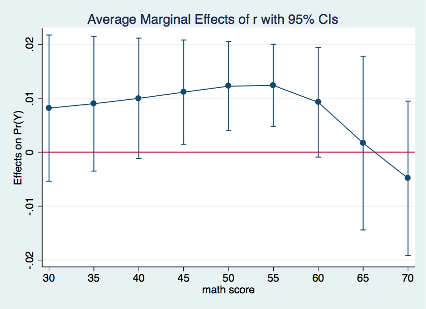
marginsplot, ylin(0)
We can make the graph more visually attractive by recasting the confidence intervals as a shaded area.
marginsplot, recast(line) recastci(rarea) ylin(0)
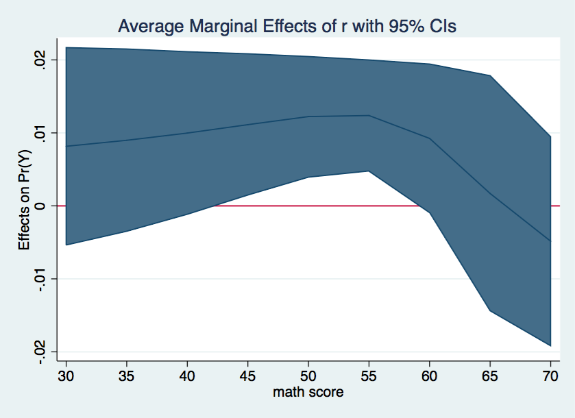
From inspection of the margins results and the graph shown above we can see that the marginal effect is statistically significant between m values of 45 to 55 inclusive. The marginal effects tells the change in probability for a one unit change in the predictor, in this case, r.
Continuous by continuous interaction with covariate
Now, let’s add a covariate, cv1 to the model. The interesting thing about logistic regression is that the marginal effects for the interaction depend on the values of the covariate even if the covariate is not part of the interaction itself. Below we show the logistic regression model with the covariate cv1 added. Because we used the parmest program previously, we will need to reload the data.
use https://stats.idre.ucla.edu/stat/data/logitconcon, clear

logit y c.r##c.m cv1, nolog

Logistic regression                               Number of obs   =        200
                                                  LR chi2(4)      =      66.80
                                                  Prob > chi2     =     0.0000
Log likelihood = -77.953857                       Pseudo R2       =     0.3000

------------------------------------------------------------------------------
           y |      Coef.   Std. Err.      z    P>|z|     [95% Conf. Interval]
-------------+----------------------------------------------------------------
           r |   .4342063   .1961642     2.21   0.027     .0497316    .8186809
           m |   .5104617   .2011856     2.54   0.011     .1161452    .9047782
             |
     c.r#c.m |  -.0068144   .0033337    -2.04   0.041    -.0133483   -.0002805
             |
         cv1 |   .0309685   .0271748     1.14   0.254    -.0222931      .08423
       _cons |  -34.09122   11.73402    -2.91   0.004    -57.08947   -11.09297
------------------------------------------------------------------------------
This time, everything except for the covariate is statistically significant. As it turns out, it doesn’t matter whether the covariate is significant or not; we still have to take the value of the covariate into account when interpreting the interaction.
Before obtaining the marginal effects we will collect some information on the covariate, namely the values one standard deviation below the mean, the mean, and one standard deviation above the mean.
summarize cv1

    Variable |       Obs        Mean    Std. Dev.       Min        Max
-------------+--------------------------------------------------------
         cv1 |       200      52.405    10.73579         26         71

display r(mean)-r(sd) "  " r(mean) "  " r(mean)+r(sd)

41.669207  52.405  63.140793
Now, we can go ahead and run the margins command including each of the three values of cv1.
/* holding cv1 at mean minus 1 sd */

margins, dydx(r) at(m=(30(5)70) cv1=(41.669207  52.405  63.140793)) vsquish noatlegend

Average marginal effects                          Number of obs   =        200
Model VCE    : OIM

Expression   : Pr(y), predict()
dy/dx w.r.t. : r

------------------------------------------------------------------------------
             |            Delta-method
             |      dy/dx   Std. Err.      z    P>|z|     [95% Conf. Interval]
-------------+----------------------------------------------------------------
r            |
         _at |
          1  |   .0061133   .0065712     0.93   0.352     -.006766    .0189926
          2  |   .0074917   .0069416     1.08   0.280    -.0061135    .0210969
          3  |   .0090189   .0073769     1.22   0.221    -.0054396    .0234774
          4  |    .006587   .0061377     1.07   0.283    -.0054427    .0186167
          5  |   .0081075   .0063953     1.27   0.205     -.004427    .0206421
          6  |   .0097902   .0067546     1.45   0.147    -.0034485    .0230289
          7  |   .0071815   .0056839     1.26   0.206    -.0039586    .0183217
          8  |   .0088605   .0057648     1.54   0.124    -.0024384    .0201593
          9  |   .0107094   .0060155     1.78   0.075    -.0010807    .0224994
         10  |   .0078851   .0052656     1.50   0.134    -.0024354    .0182055
         11  |    .009721   .0051157     1.90   0.057    -.0003056    .0197476
         12  |   .0117184   .0052384     2.24   0.025     .0014513    .0219854
         13  |   .0085235    .004981     1.71   0.087    -.0012391    .0182861
         14  |   .0104242   .0046175     2.26   0.024     .0013739    .0194744
         15  |   .0124196   .0046088     2.69   0.007     .0033864    .0214527
         16  |   .0083341   .0049614     1.68   0.093    -.0013901    .0180583
         17  |     .00992   .0046688     2.12   0.034     .0007692    .0190708
         18  |   .0114027    .004686     2.43   0.015     .0022182    .0205871
         19  |   .0052692   .0059747     0.88   0.378    -.0064411    .0169795
         20  |   .0058498    .006339     0.92   0.356    -.0065745    .0182741
         21  |    .006181   .0067253     0.92   0.358    -.0070003    .0193622
         22  |   -.002175   .0090427    -0.24   0.810    -.0198984    .0155484
         23  |  -.0021432   .0088189    -0.24   0.808     -.019428    .0151416
         24  |  -.0020011   .0080879    -0.25   0.805    -.0178531    .0138509
         25  |  -.0091967   .0089699    -1.03   0.305    -.0267774    .0083839
         26  |  -.0081533   .0075364    -1.08   0.279    -.0229243    .0066177
         27  |  -.0069432   .0060361    -1.15   0.250    -.0187739    .0048874
------------------------------------------------------------------------------
It is difficult to make sense out of all of the numbers in the above table. Plotting the results will aid us in interpreting the margins results. Using the by option with marginsplot will get us three plot, one for each of the three values of cv1.
marginsplot, by(cv1) yline(0)
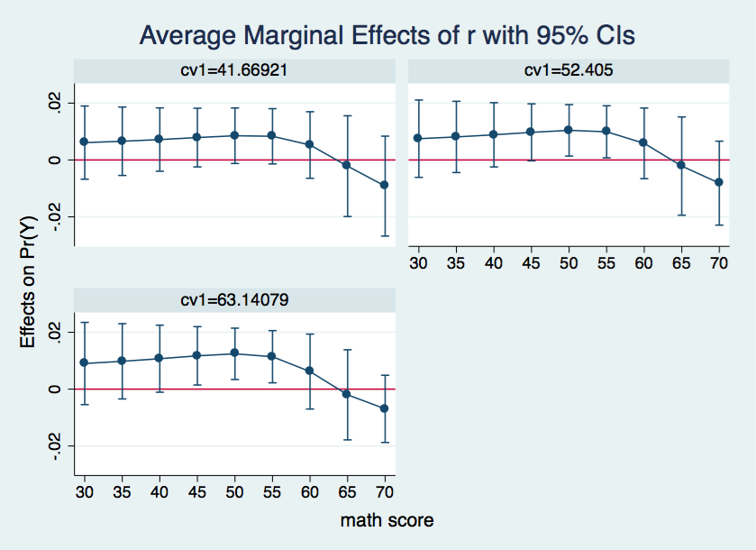
Looking at the three plots of margins results we see that when the covariate is one standard deviation below the mean there are no significant marginal effects. When the covariate is held at it mean value then the marginal effects for m at 50 and 55 are
significant. And, finally when the covariate is held at the mean plus one standard deviation then the marginal effect for r is statistically significant when m is between 45 and 55.
It might be useful to look at a single graph combining all three plots. In fact, we’ll go all out and include shaded confidence intervals.
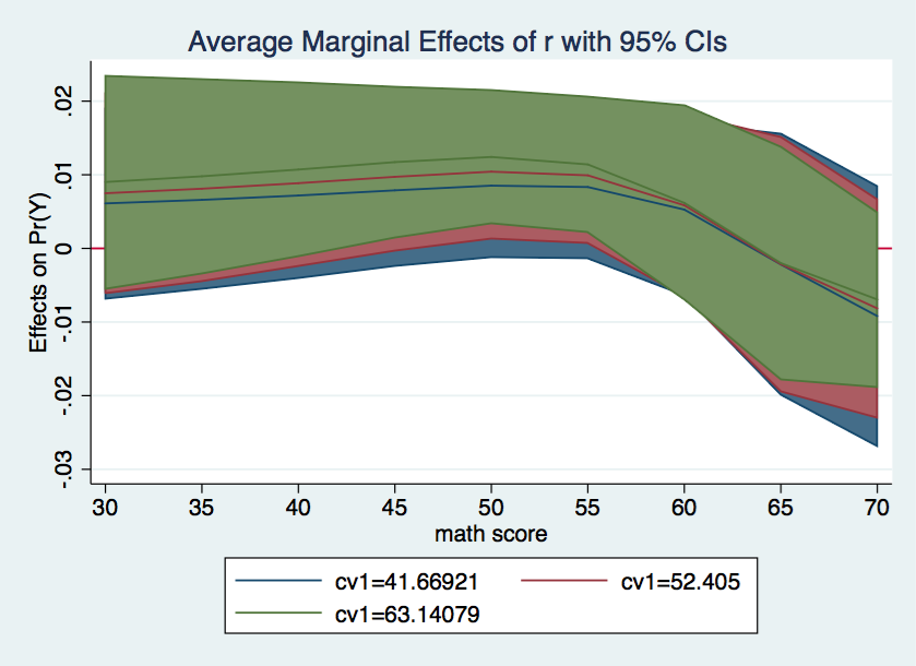
Nice graph, but I don’t know if it really makes the results easier to interpret.