Let’s begin with with what a significant three-way interaction means. It means that there is a two-way interaction that varies across levels of a third variable. Say, for example, that a b#c interaction differs across various levels of factor a.
One way of analyzing the three-way interaction is to begin by testing two-way interactions at each level of a third variable. This process is just a generalization of tests of simple effects which can is used for two-way interactions. If you find the material on this FAQ page to be confusing there is another page which takes a more conceptual approach that is not stat package specific. That page is located here.
We will use a small artificial example that has a statistically significant three-way interaction to illustrate the process.
use https://stats.idre.ucla.edu/stat/stata/faq/threeway, clear

anova y a##b##c

                           Number of obs =      24     R-squared     =  0.9689
                           Root MSE      =  1.1547     Adj R-squared =  0.9403

                  Source |  Partial SS    df       MS           F     Prob > F
              -----------+----------------------------------------------------
                   Model |  497.833333    11  45.2575758      33.94     0.0000
                         |
                       a |         150     1         150     112.50     0.0000
                       b |  .666666667     1  .666666667       0.50     0.4930
                       c |  127.583333     2  63.7916667      47.84     0.0000
                     a#b |  160.166667     1  160.166667     120.12     0.0000
                     a#c |       18.25     2       9.125       6.84     0.0104
                     b#c |  22.5833333     2  11.2916667       8.47     0.0051
                   a#b#c |  18.5833333     2  9.29166667       6.97     0.0098
                         |
                Residual |          16    12  1.33333333
              -----------+----------------------------------------------------
                   Total |  513.833333    23  22.3405797
Next, we’ll look at the cell means using the margins command.
margins a#b#c

Adjusted predictions                              Number of obs   =         24

Expression   : Linear prediction, predict()

------------------------------------------------------------------------------
             |            Delta-method
             |     Margin   Std. Err.      z    P>|z|     [95% Conf. Interval]
-------------+----------------------------------------------------------------
       a#b#c |
      1 1 1  |         11   .8164966    13.47   0.000     9.399696     12.6003
      1 1 2  |         15   .8164966    18.37   0.000      13.3997     16.6003
      1 1 3  |         19   .8164966    23.27   0.000      17.3997     20.6003
      1 2 1  |       10.5   .8164966    12.86   0.000     8.899696     12.1003
      1 2 2  |       10.5   .8164966    12.86   0.000     8.899696     12.1003
      1 2 3  |        9.5   .8164966    11.64   0.000     7.899696     11.1003
      2 1 1  |       10.5   .8164966    12.86   0.000     8.899696     12.1003
      2 1 2  |       15.5   .8164966    18.98   0.000      13.8997     17.1003
      2 1 3  |       18.5   .8164966    22.66   0.000      16.8997     20.1003
      2 2 1  |       16.5   .8164966    20.21   0.000      14.8997     18.1003
      2 2 2  |       20.5   .8164966    25.11   0.000      18.8997     22.1003
      2 2 3  |         24   .8164966    29.39   0.000      22.3997     25.6003
------------------------------------------------------------------------------
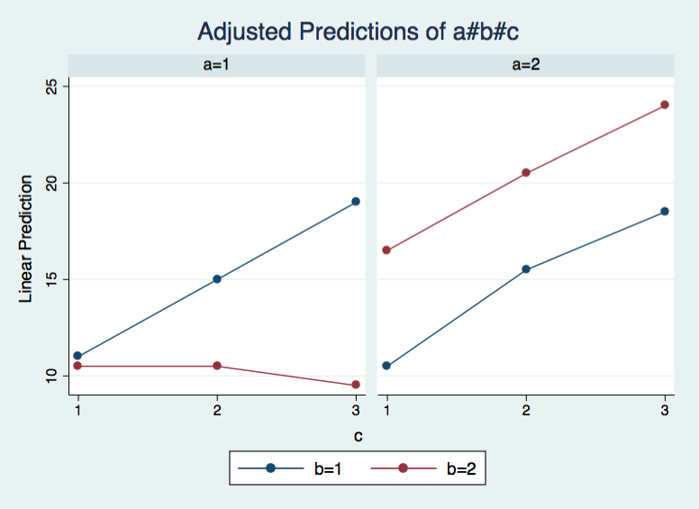
Next, we will plot the cells means to see which effects look promising to follow up on. The marginsplot command will do the job for us.
marginsplot, by(a) x(c) noci
We believe from looking at the graph above that the three-way interaction is significant because there appears to be a “strong” two-way interaction at a = 1 and no interaction at a = 2. Now, we just have to show it statistically using tests of simple effects. To do this we will use the contrast command. The b#a@a, in the command, looks a little strange but it is just requesting the b#c interaction effect for each level of variable a.
contrast b#c@a

Contrasts of marginal linear predictions

Margins      : asbalanced

------------------------------------------------
             |         df           F        P>F
-------------+----------------------------------
       b#c@a |
          1  |          2       15.25     0.0005
          2  |          2        0.19     0.8314
      Joint  |          4        7.72     0.0026
             |
    Residual |         12
------------------------------------------------
The F-ratio for the b#c interaction at a = 1 is 15.25, while the F-ratio for the b#c at a =2 is 0.19. The p-values given in the table have not been adjusted for these post-hoc multiple comparisons. This is a topic we need to discuss.
Clearly, one F-ratio is much larger than the other but how can we tell which are statistically significant? There are at least four different methods of determining the critical value of tests of simple main-effects. There is a method related to Dunn’s multiple comparisons, a method attributed to Marascuilo & Levin, a method called the simultaneous test procedure (very conservative and related to the Scheffé post-hoc test) and a per family error rate method.
We will demonstrate the per family error rate method but you should look up the other methods in a good anova book, like Kirk (1995), to decide which approach is best for your situation. The trick here is that we divide 0.05, our alpha level, by 2 in the invfprob function because we are doing two tests of simple main-effects.
/* compute critical value */
display "critical value per family error rate = " invfprob(2, 12, 0.05/2)

critical value per family error rate = 5.0958672
The critical value is approximately 5.1. The first F-ratio of 15.25 is significant while the second (.1875) is not. In other words, the two-way b#c interaction is significant at a = 1 but is not significant at a = 2.
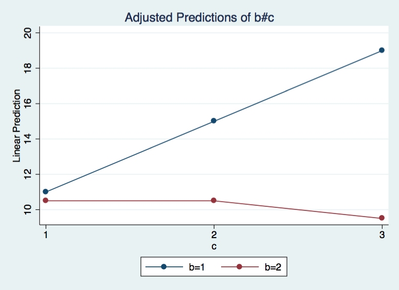
In an ideal world we would be done now, but since we live in the “real” world, there is still more to do because we now need to try to understand the significant two-way interaction at a = 1; first for b = 1 and then for b = 2. Let’s remake the plot of the cell means for b and c at a = 1.
margins b#c, at(a=1)

Adjusted predictions                              Number of obs   =         24

Expression   : Linear prediction, predict()
at           : a               =           1

------------------------------------------------------------------------------
             |            Delta-method
             |     Margin   Std. Err.      z    P>|z|     [95% Conf. Interval]
-------------+----------------------------------------------------------------
         b#c |
        1 1  |         11   .8164966    13.47   0.000     9.399696     12.6003
        1 2  |         15   .8164966    18.37   0.000      13.3997     16.6003
        1 3  |         19   .8164966    23.27   0.000      17.3997     20.6003
        2 1  |       10.5   .8164966    12.86   0.000     8.899696     12.1003
        2 2  |       10.5   .8164966    12.86   0.000     8.899696     12.1003
        2 3  |        9.5   .8164966    11.64   0.000     7.899696     11.1003
------------------------------------------------------------------------------

marginsplot, x(c) noci

To perform the next test we could use the margins command with the contrast option. Here’s what it looks like.
margins c@b, at(a=1) contrast

Contrasts of adjusted predictions

Expression   : Linear prediction, predict()
at           : a               =           1

------------------------------------------------
             |         df        chi2     P>chi2
-------------+----------------------------------
         c@b |
          1  |          2       48.00     0.0000
          2  |          2        1.00     0.6065
      Joint  |          4       49.00     0.0000
------------------------------------------------
You will note that the margins, contrast command displays the test statistic as a chi-square not as an F-ratio. If we use the contrast command the test statistic will be scaled as an F-ratio. The trick to getting the command to work for this analysis is to use the @ symbol twice, once with b and once with i(1).a.
contrast c@b@i(1).a

Contrasts of marginal linear predictions

Margins      : asbalanced

------------------------------------------------
             |         df           F        P>F
-------------+----------------------------------
       c@b#a |
        1 1  |          2       24.00     0.0001
        2 1  |          2        0.50     0.6186
      Joint  |          4       12.25     0.0003
             |
 Denominator |         12
------------------------------------------------
Only the test of simple effects of c at b = 1 was statistically significant. But we’re not done yet, since there are three levels of c, we don’t know where this significant effect lies. We need to test the pairwise comparisons among the three means when b = 1 and a = 1. We will do this using the the pwcompare command (introduced in Stata 12) with the mcompare(tukey) and effect options.
pwcompare c#i(1).b#i(1).a, mcompare(tukey) effects

Pairwise comparisons of marginal linear predictions

Margins      : asbalanced

---------------------------
             |    Number of
             |  Comparisons
-------------+-------------
       c#b#a |            3
---------------------------

-------------------------------------------------------------------------------------
                    |                              Tukey                Tukey
                    |   Contrast   Std. Err.      t    P>|t|     [95% Conf. Interval]
--------------------+----------------------------------------------------------------
              c#b#a |
(2 1 1) vs (1 1 1)  |          4   1.154701     3.46   0.012     .9194165    7.080584
(3 1 1) vs (1 1 1)  |          8   1.154701     6.93   0.000     4.919416    11.08058
(3 1 1) vs (2 1 1)  |          4   1.154701     3.46   0.012     .9194165    7.080584
-------------------------------------------------------------------------------------
From the table above, it appears that all three of the pairwise comparisons are statistically significant.
The process would have be similar if we had chosen a different two-way interaction back at the beginning.
One final note, all of the commands shown on this page work exactly the same if we had run the model using regress instead of anova.
Summary of Steps
1) Run full model with three-way interaction. 1a) Capture SS and df residual. 2) Run two-way interaction at each level of third variable. 2a) Capture SS and df for interactions. 2b) Compute F-ratios for tests of interaction at levels of a 3rd variable. 3) Run one-way model at each level of second variable. 3a) Capture SS and df for main effects. 3b) Compute F-ratios for tests of simple main-effects. 4) Run pairwise or other post-hoc comparisons if necessary
References
Kirk, Roger E. (1995) Experimental Design: Procedures for the Behavioral Sciences, Third Edition. Monterey, California: Brooks/Cole Publishing.

