The margins command, new in Stata 11, can be a very useful tool in understanding and interpreting interactions. We will illustrate the command for a logistic regression model with two categorical by continuous interactions. We begin by loading the dataset mlogcatcon.
use https://stats.idre.ucla.edu/stat/data/mlogcatcon, clear
In this dataset y is the binary response variable and m and s are continuous predictors. The variable f, which stands for female, is a binary predictor. We will interact f with both m and s. Here is the logistic regression model.
logit y f##c.m f##c.s

Iteration 0:   log likelihood = -109.04953
...
Iteration 5:   log likelihood = -69.533946

Logistic regression                               Number of obs   =        200
                                                  LR chi2(5)      =      79.03
                                                  Prob > chi2     =     0.0000
Log likelihood = -69.533946                       Pseudo R2       =     0.3624

------------------------------------------------------------------------------
           y |      Coef.   Std. Err.      z    P>|z|     [95% Conf. Interval]
-------------+----------------------------------------------------------------
         1.f |  -11.64885    5.31706    -2.19   0.028     -22.0701   -1.227609
           m |   .0907151   .0348589     2.60   0.009      .022393    .1590372
             |
       f#c.m |
          1  |   .0426602   .0577991     0.74   0.460     -.070624    .1559445
             |
           s |    .074839   .0330348     2.27   0.023      .010092    .1395859
             |
       f#c.s |
          1  |   .1471401   .0725369     2.03   0.043     .0049704    .2893098
             |
       _cons |   -10.1233   2.323433    -4.36   0.000    -14.67714   -5.569451
------------------------------------------------------------------------------
You will note that the f by s interaction is statistically significant while the f by m interaction is not. Since this is a nonlinear model we will have to take the values of all covariates into account in understanding what is going on in the model.
We will start with a margins command that looks at the discrete difference in probability between males and females for five different levels of s while holding m at its mean value. We get the discrete difference in probability using the dydx option with the binary predictor. The variable m will be held at its mean value using the atmeans option.
margins, dydx(f) at(s=(30(10)70)) atmeans noatlegend

Conditional marginal effects                      Number of obs   =        200
Model VCE    : OIM

Expression   : Pr(y), predict()
dy/dx w.r.t. : 1.f

------------------------------------------------------------------------------
             |            Delta-method
             |      dy/dx   Std. Err.      z    P>|z|     [95% Conf. Interval]
-------------+----------------------------------------------------------------
1.f          |
         _at |
          1  |   -.042701   .0367882    -1.16   0.246    -.1148046    .0294026
          2  |  -.0839342   .0472826    -1.78   0.076    -.1766064    .0087379
          3  |  -.1419013   .0533704    -2.66   0.008    -.2465053   -.0372973
          4  |  -.1051027   .0980072    -1.07   0.284    -.2971932    .0869878
          5  |   .2145781   .2161073     0.99   0.321    -.2089845    .6381407
------------------------------------------------------------------------------
Note: dy/dx for factor levels is the discrete change from the base level.
While the results of the margins command above are perfectly correct, they reflect the discrete change in probability for only a single value of m. If we remove the atmeans option we get the average marginal effect, i.e., the discrete change in probability for each of the values of s averaged across the observed values of m. Here is how the margins command looks now.
margins, dydx(f) at(s=(30(10)70)) noatlegend

Average marginal effects                          Number of obs   =        200
Model VCE    : OIM

Expression   : Pr(y), predict()
dy/dx w.r.t. : 1.f

------------------------------------------------------------------------------
             |            Delta-method
             |      dy/dx   Std. Err.      z    P>|z|     [95% Conf. Interval]
-------------+----------------------------------------------------------------
1.f          |
         _at |
          1  |  -.0575153   .0497762    -1.16   0.248    -.1550748    .0400441
          2  |  -.1048622   .0581838    -1.80   0.072    -.2189004     .009176
          3  |   -.148558   .0594204    -2.50   0.012    -.2650197   -.0320962
          4  |  -.0726804   .0766543    -0.95   0.343    -.2229201    .0775593
          5  |   .1663325   .1894277     0.88   0.380     -.204939     .537604
------------------------------------------------------------------------------
Note: dy/dx for factor levels is the discrete change from the base level.
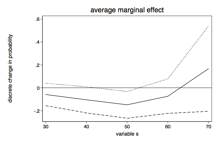
Let’s go ahead and graph these results including the 95% confidence intervals. We will begin by placing placing necessary values into a matrix using techniques shown in Stata FAQ: How can I graph the results of the margins command?. The matrix commands will be followed by a twoway line graph.
matrix b=r(b)'
matrix b=b[6...,1]
matrix m=r(at)
matrix m=m[1...,4]
matrix v=r(V)
matrix v=v[6...,6...]
matrix se=vecdiag(cholesky(diag(vecdiag(v))))'
matrix ll=b-1.96*se
matrix ul=b+1.96*se

matrix m=m,b,ll,ul

matrix list m

m[5,4]
             s          r1          r1          r1
r1          30  -.05751532  -.15507658   .04004594
r2          40  -.10486222  -.21890253   .00917809
r3          50  -.14855797  -.26502187  -.03209408
r4          60  -.07268039  -.22292282   .07756203
r5          70   .16633254  -.20494579   .53761086

svmat m

twoway line m2 m3 m4 m1, scheme(lean1) legend(off) yline(0) ///
       ytitle(discrete change in probability) xtitle(variable s) ///
       title(average marginal effect) name(ame, replace)


drop m1-m4 /* drop these variables -- they are no longer needed */
The margins command and the graph above give us a pretty good idea of how the discrete change in probability varies across different values of s but we still don’t know how this changes with differing values of m. Let’s try the margins command once more, this time varying both s and m.
margins, dydx(f) at(s=(30(10)70) m=(30(10)70)) vsquish

Conditional marginal effects                      Number of obs   =        200
Model VCE    : OIM

Expression   : Pr(y), predict()
dy/dx w.r.t. : 1.f
1._at        : m               =          30
               s               =          30
2._at        : m               =          30
               s               =          40
3._at        : m               =          30
               s               =          50
4._at        : m               =          30
               s               =          60
5._at        : m               =          30
               s               =          70
6._at        : m               =          40
               s               =          30
7._at        : m               =          40
               s               =          40
8._at        : m               =          40
               s               =          50
9._at        : m               =          40
               s               =          60
10._at       : m               =          40
               s               =          70
11._at       : m               =          50
               s               =          30
12._at       : m               =          50
               s               =          40
13._at       : m               =          50
               s               =          50
14._at       : m               =          50
               s               =          60
15._at       : m               =          50
               s               =          70
16._at       : m               =          60
               s               =          30
17._at       : m               =          60
               s               =          40
18._at       : m               =          60
               s               =          50
19._at       : m               =          60
               s               =          60
20._at       : m               =          60
               s               =          70
21._at       : m               =          70
               s               =          30
22._at       : m               =          70
               s               =          40
23._at       : m               =          70
               s               =          50
24._at       : m               =          70
               s               =          60
25._at       : m               =          70
               s               =          70

------------------------------------------------------------------------------
             |            Delta-method
             |      dy/dx   Std. Err.      z    P>|z|     [95% Conf. Interval]
-------------+----------------------------------------------------------------
1.f          |
         _at |
          1  |  -.0057129   .0063763    -0.90   0.370    -.0182102    .0067844
          2  |  -.0118921   .0116175    -1.02   0.306    -.0346619    .0108777
          3  |  -.0238252   .0229579    -1.04   0.299    -.0688218    .0211714
          4  |  -.0400685   .0516074    -0.78   0.438    -.1412171    .0610802
          5  |  -.0062295   .1691796    -0.04   0.971    -.3378154    .3253565
          6  |  -.0140135   .0131539    -1.07   0.287    -.0397946    .0117675
          7  |  -.0287583   .0208235    -1.38   0.167    -.0695717     .012055
          8  |  -.0551503   .0356445    -1.55   0.122    -.1250121    .0147116
          9  |  -.0763916   .0804218    -0.95   0.342    -.2340155    .0812323
         10  |   .0676689   .2718875     0.25   0.803    -.4652207    .6005586
         11  |  -.0339307   .0292713    -1.16   0.246    -.0913013    .0234399
         12  |  -.0675498   .0389036    -1.74   0.083    -.1437994    .0086999
         13  |  -.1184831   .0480101    -2.47   0.014    -.2125811    -.024385
         14  |  -.1065329    .097911    -1.09   0.277     -.298435    .0853692
         15  |   .1934334   .2441036     0.79   0.428    -.2850009    .6718678
         16  |    -.07971   .0710032    -1.12   0.262    -.2188738    .0594538
         17  |  -.1487312   .0866721    -1.72   0.086    -.3186054     .021143
         18  |  -.2164891   .0908541    -2.38   0.017    -.3945598   -.0384185
         19  |  -.0634788    .110638    -0.57   0.566    -.2803254    .1533677
         20  |   .2182539   .1473218     1.48   0.138    -.0704916    .5069993
         21  |  -.1751863   .1667445    -1.05   0.293    -.5019995    .1516269
         22  |  -.2866478   .1890498    -1.52   0.129    -.6571787     .083883
         23  |  -.2841612   .2168233    -1.31   0.190     -.709127    .1408047
         24  |   .0354487   .1731142     0.20   0.838    -.3038489    .3747462
         25  |   .1446316   .1002235     1.44   0.149    -.0518029    .3410661
------------------------------------------------------------------------------
Note: dy/dx for factor levels is the discrete change from the base level.
The first five rows give the discrete change for the five values of s while holding m at 30. The next five hold m at 40. And so on. One of the more interesting features is how few of the discrete changes are statistically significant even though the overall f by s interaction was significant.
Now we can collect the necessary values into a matrix in preparation for graphing.
matrix m=r(at)
matrix m=m[1...,3..4]
matrix b=r(b)'
matrix b=b[26...,1]
matrix m = m,b
matrix colnames m = mvar svar coef
matrix list m

m[25,3]
           mvar        svar        coef
 r1          30          30  -.00042464
 r2          30          40  -.00139674
 r3          30          50  -.00455224
 r4          30          60  -.01440282
 r5          30          70  -.04155818
 r6          40          30   -.0012454
 r7          40          40  -.00406479
 r8          40          50  -.01291961
 r9          40          60   -.0377978
r10          40          70  -.08770375
r11          50          30  -.00362874
r12          50          40    -.011581
r13          50          50  -.03430757
r14          50          60  -.08224427
r15          50          70   -.1233095
r16          60          30  -.01037455
r17          60          40  -.03108193
r18          60          50  -.07678675
r19          60          60  -.12194728
r20          60          70  -.10037149
r21          70          30  -.02811225
r22          70          40  -.07139767
r23          70          50  -.11982559
r24          70          60  -.10522467
r25          70          70  -.05170914

svmat m, names(col)
Let’s begin by graphing the effect of different values of s with separate lines for each value of m.
twoway (line coef svar if mvar==30)(line coef svar if mvar==40)(line coef svar if mvar==50) ///
       (line coef svar if mvar==60)(line coef svar if mvar==70), scheme(lean1) ///
       legend(order ( 1 "m30" 2 "m40" 3 "m50" 4 "m60" 5 "m70")) ///
       name(sbym, replace) xtitle(variable s) ytitle(discrete change in probability)
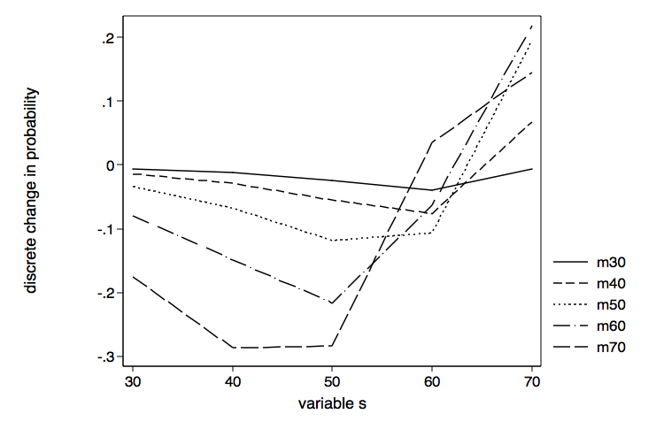
Although there were not a lot of significant values in the margins table above, the lines for each of the values of m look rather different from one another. While the line for m equal 30 is rather flat the line for m equal 70 displays a lot more variability, first dropping and then climbing steeply around s equal 50.
Now that we know what differences in s for values of m looks like, we can reverse the variables in the graphics command (twoway line) to see what differences in m for values of s looks like.
twoway (line coef mvar if svar==30)(line coef mvar if svar==40)(line coef mvar if svar==50) ///
       (line coef mvar if svar==60)(line coef mvar if svar==70), scheme(lean1) ///
       legend(order ( 1 "s30" 2 "s40" 3 "s50" 4 "s60" 5 "s70")) ///
       name(sbym, replace) xtitle(variable m) ytitle(discrete change in probability)
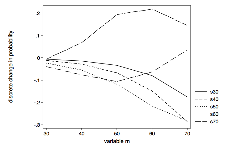
Of course, we are looking at the same 25 values as the previous graph, just organized differently. This time the line for s equal 70 is the one that stands out from the others.
If your model is more complex than this one, you have to decide what to do with each of the covariates. You can hold them constant at one or more values or you can average over them. Whatever choice you make you need to realize that the values of all of the covariates matter in nonlinear models.