The margins command, new in Stata 11, can be a very useful tool in understanding and interpreting interactions. On this page we will use margins for a three factor anova model with a significant 3-way interaction. We will illustrate this using the following dataset.
use https://stats.idre.ucla.edu/stat/stata/faq/threeway, clear
The data will be analyzed as a 2x2x3 factorial anova. Variables a and b have two levels each while variable c has three levels. We will begin by running the anova model.
anova y a##b##c   /* equivalent to: anova y a b c a#b a#c b#c a#b#c */

                           Number of obs =      24     R-squared     =  0.9689
                           Root MSE      =  1.1547     Adj R-squared =  0.9403

                  Source |  Partial SS    df       MS           F     Prob > F
              -----------+----------------------------------------------------
                   Model |  497.833333    11  45.2575758      33.94     0.0000
                         |
                       a |         150     1         150     112.50     0.0000
                       b |  .666666667     1  .666666667       0.50     0.4930
                       c |  127.583333     2  63.7916667      47.84     0.0000
                     a#b |  160.166667     1  160.166667     120.13     0.0000
                     a#c |       18.25     2       9.125       6.84     0.0104
                     b#c |  22.5833333     2  11.2916667       8.47     0.0051
                   a#b#c |  18.5833333     2  9.29166667       6.97     0.0098
                         |
                Residual |          16    12  1.33333333
              -----------+----------------------------------------------------
                   Total |  513.833333    23  22.3405797
Indeed, it is the case that the 3-way interaction is statistically significant. Here is the plan for interpreting this interaction. First, we will run the margins command with the asbalanced option on the interaction term to get adjusted cell means. In this case the design already is balanced but the asbalanced option is included for those cases in which the data are unbalanced so that we don’t forget it. We will also use the post option because we are planning on doing tests among the cell means.
The significant 3-way interaction suggests that there are one or more two-way interactions that are significant. We will select some two-way interactions to test for each of the levels of the third variable. If any of the two-way interactions are significant we will test the main effect of one variable at each level of the other variable. These are known as tests of simple main effects. Finally, if necessary, we follow these tests of simple main effects up with pair-wise comparisons among the appropriate means.
Here is the margins command.
margins a#b#c, post asbalanced

Adjusted predictions                              Number of obs   =         24

Expression   : Linear prediction, predict()

------------------------------------------------------------------------------
             |            Delta-method
             |     Margin   Std. Err.      z    P>|z|     [95% Conf. Interval]
-------------+----------------------------------------------------------------
       a#b#c |
      1 1 1  |         11   .8164966    13.47   0.000     9.399696     12.6003
      1 1 2  |         15   .8164966    18.37   0.000      13.3997     16.6003
      1 1 3  |         19   .8164966    23.27   0.000      17.3997     20.6003
      1 2 1  |       10.5   .8164966    12.86   0.000     8.899696     12.1003
      1 2 2  |       10.5   .8164966    12.86   0.000     8.899696     12.1003
      1 2 3  |        9.5   .8164966    11.64   0.000     7.899696     11.1003
      2 1 1  |       10.5   .8164966    12.86   0.000     8.899696     12.1003
      2 1 2  |       15.5   .8164966    18.98   0.000      13.8997     17.1003
      2 1 3  |       18.5   .8164966    22.66   0.000      16.8997     20.1003
      2 2 1  |       16.5   .8164966    20.21   0.000      14.8997     18.1003
      2 2 2  |       20.5   .8164966    25.11   0.000      18.8997     22.1003
      2 2 3  |         24   .8164966    29.39   0.000      22.3997     25.6003
------------------------------------------------------------------------------
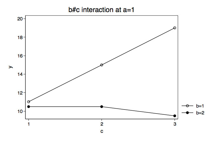
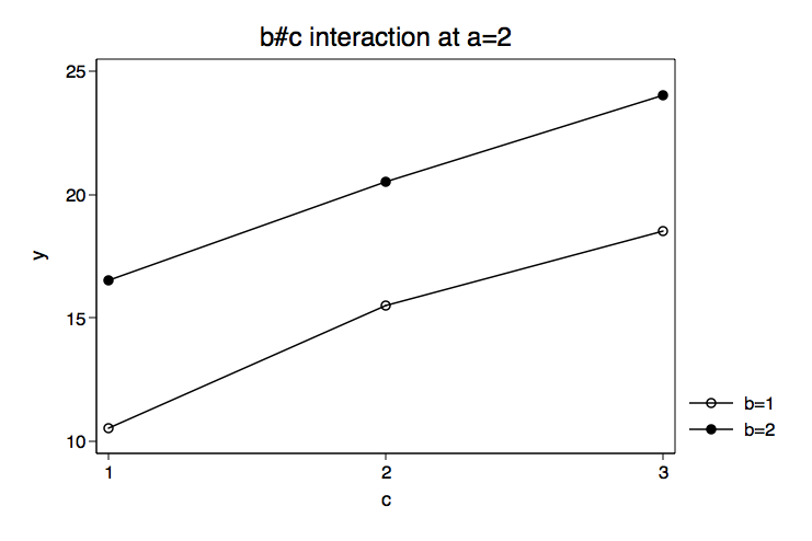
Because we have some specific prior knowledge concerning the variables in this model we will begin by plotting the cell means for the b by c interactions for each level of a. We do this by putting the estimates from the margins command into a matrix mean. Then we create separate matrices for the levels of the three factor variables, cleverly calling them a, b and c. You can look at any of these matrices by typing matrix list followed by the matrix name. We will combine all of the matrices together into a matrix called gph. Using the svmat command we will put the matrix values into out data in memory. Finally, we will plot the means using the twoway line command twice, once for each b#c interaction.
/* you can look at any of these matrices by using matrix list matname */

matrix means=e(b)'

/* note: # is the kronecker product operator */

matrix gpha=(12)#(111111)  /* levels of a */

matrix gphb=(1212)#(111)    /* levels of b */

matrix gphc=(1111)#(123)    /* levels of c */

/* put them all together */
matrix gph= gpha,gphb,gphc,means

matrix list gph

gph[12,4]
          c1:   c1:   c1:
          c1    c1    c1    y1
 r1:r1     1     1     1    11
 r1:r2     1     1     2    15
 r1:r3     1     1     3    19
 r1:r4     1     2     1  10.5
 r1:r5     1     2     2  10.5
 r1:r6     1     2     3   9.5
 r2:r7     2     1     1  10.5
 r2:r8     2     1     2  15.5
 r2:r9     2     1     3  18.5
r2:r10     2     2     1  16.5
r2:r11     2     2     2  20.5
r2:r12     2     2     3    24

svmat gph

twoway (connect gph4 gph3 if gph1==1 & gph2==1)(connect gph4 gph3 if gph1==1 & gph2==2), ///
       legend(order(1 "b=1" 2 "b=2")) ytitle(y) xtitle(c) xlabel(1 2 3) ///
       title("b#c interaction at a=1") name(bc_at_a1, replace) scheme(lean1)


twoway (connect gph4 gph3 if gph1==2 & gph2==1)(connect gph4 gph3 if gph1==2 & gph2==2), ///
       legend(order(1 "b=1" 2 "b=2")) ytitle(y) xtitle(c) xlabel(1 2 3) ///
       title("b#c interaction at a=2") name(bc_at_a2, replace) scheme(lean1)

The graphs of the cell means suggest that the b#c interaction at a=1 will be significant while the b#c interaction at a=2 will not. We will use the test command to test the two-way interactions at for each level of a. These tests are two degrees of freedom each and will refer to specific cell means with correct signs to get an interaction effect. Essentially, we are specifying a two-way interaction using just the cell means. This is not difficult to set up especially if we use a table representing the six cells and plus with minuses to indicate the appropriate signs. Here is the table for the first degree of freedom.
    c1  c2  c3
b1   +   -
b2   -   +
The second degree of freedom refers to this next table.
    c1  c2  c3
b1   +       -
b2   -       +
These two tables translate into the test commands shown below. Each part of the test command inside parentheses is one degree of freedom.
To simplify adjustments for multiple testing we will use a Bonferroni adjustment across all tests of simple main effects and pair-wise comparisons. Having already run through this analysis before writing this web page, I know that there will be seven such tests. Therefore I have included a display command giving the adjusted p-values for each test.
/* tests of b#c for each level of a */

/* test of b#c at a=1 */
test (1.a#1.b#1.c - 1.a#1.b#2.c - 1.a#2.b#1.c + 1.a#2.b#2.c = 0) ///
     (1.a#1.b#1.c - 1.a#1.b#3.c - 1.a#2.b#1.c + 1.a#2.b#3.c = 0)

 ( 1)  1bn.a#1bn.b#1bn.c - 1bn.a#1bn.b#2.c - 1bn.a#2.b#1bn.c + 1bn.a#2.b#2.c = 0
 ( 2)  1bn.a#1bn.b#1bn.c - 1bn.a#1bn.b#3.c - 1bn.a#2.b#1bn.c + 1bn.a#2.b#3.c = 0

           chi2(  2) =   30.50
         Prob > chi2 =    0.0000

display "Bonferroni adjusted p-value: " %7.6f r(p)*7

Bonferroni adjusted p-value: 0.000002

/* test of b#c at a=2 */
test (2.a#1.b#1.c - 2.a#1.b#2.c - 2.a#2.b#1.c + 2.a#2.b#2.c = 0) ///
     (2.a#1.b#1.c - 2.a#1.b#3.c - 2.a#2.b#1.c + 2.a#2.b#3.c = 0)

 ( 1)  2.a#1bn.b#1bn.c - 2.a#1bn.b#2.c - 2.a#2.b#1bn.c + 2.a#2.b#2.c = 0
 ( 2)  2.a#1bn.b#1bn.c - 2.a#1bn.b#3.c - 2.a#2.b#1bn.c + 2.a#2.b#3.c = 0

           chi2(  2) =    0.38
         Prob > chi2 =    0.8290

display "Bonferroni adjusted p-value: " %7.6f r(p)*7

Bonferroni adjusted p-value: 5.803204
Our guess from looking at the graph of the cell means was correct. The test of b#c at a=1 was significant while b#c at a=2 was not. We can follow this up with tests of differences among levels of c for each level of b while holding a at one. Each of these tests will also have two degrees of freedom
/* tests of c for each level of b at a=1 */

/* test of c at b=1 & a=1 */
test (1.a#1.b#1.c - 1.a#1.b#2.c = 0)(1.a#1.b#1.c - 1.a#1.b#3.c = 0)

 ( 1)  1bn.a#1bn.b#1bn.c - 1bn.a#1bn.b#2.c = 0
 ( 2)  1bn.a#1bn.b#1bn.c - 1bn.a#1bn.b#3.c = 0

           chi2(  2) =   48.00
         Prob > chi2 =    0.0000

display "Bonferroni adjusted p-value: " %7.6f r(p)*7

Bonferroni adjusted p-value: 0.000000

/* test of c at b=2 & a=2 */
test (1.a#2.b#1.c - 1.a#2.b#2.c = 0)(1.a#2.b#1.c - 1.a#2.b#3.c = 0)

 ( 1)  1bn.a#2.b#1bn.c - 1bn.a#2.b#2.c = 0
 ( 2)  1bn.a#2.b#1bn.c - 1bn.a#2.b#3.c = 0

           chi2(  2) =    1.00
         Prob > chi2 =    0.6065

display "Bonferroni adjusted p-value: " %7.6f r(p)*7

Bonferroni adjusted p-value: 4.245715
The test for differences among levels of c for b=1 while holding a at one was significant. We will follow this significant test up by looking at all pair-wise comparisons among the levels of c for b=1 and a=1. Each of these tests uses one degree of freedom.
/* all pairwise comparisons between levels of c at b=1 a=1 */

test 1.a#1.b#1.c = 1.a#1.b#2.c  /* c1 vs c2 */

 ( 1)  1bn.a#1bn.b#1bn.c - 1bn.a#1bn.b#2.c = 0

           chi2(  1) =   12.00
         Prob > chi2 =    0.0005

display "Bonferroni adjusted p-value: " %7.6f r(p)*7

Bonferroni adjusted p-value: 0.003724

test 1.a#1.b#1.c = 1.a#1.b#3.c  /* c1 vs c3 */

 ( 1)  1bn.a#1bn.b#1bn.c - 1bn.a#1bn.b#3.c = 0

           chi2(  1) =   48.00
         Prob > chi2 =    0.0000

display "Bonferroni adjusted p-value: " %7.6f r(p)*7

Bonferroni adjusted p-value: 0.000000

test 1.a#1.b#2.c = 1.a#1.b#3.c  /* c2 vs c3 */

 ( 1)  1bn.a#1bn.b#2.c - 1bn.a#1bn.b#3.c = 0

           chi2(  1) =   12.00
         Prob > chi2 =    0.0005

display "Bonferroni adjusted p-value: "%7.6f r(p)*7

Bonferroni adjusted p-value: 0.003724
It appears that each of the pair-wise comparisons among levels of c for b=1 and a=1. Thus, we have finally reached the end of our journey and are hopefully more informed then at the beginning.
