When analyzing geospatial data, describing the spatial pattern of a measured variable is of great importance. User written Stata commands allow you to explore such patterns. This page will use the variog and variog2 command. To install this, type search variog in your command window.
The variog command allows you to calculate and graph a variogram for regularly spaced one-dimensional data. The variog2 command allows you to calculate and graph a variogram for two-dimensional data without constraints on spacing. In both cases, the variogram illustrates how differences in a measured variable Z vary as the distances between the points at which Z is measured increase.
Let’s look at an example. Our dataset contains ozone measurements from thirty-two locations in the Los Angeles area aggregated over one month. The dataset includes the station number (station), the latitude and longitude of the station (lat and lon), and the average of the highest eight hour daily averages (av8top). This data, and other spatial datasets, can be downloaded from the GeoDa Center for Geospatial Analysis and Computation.
use https://stats.idre.ucla.edu/stat/stata/faq/ozone, clear
clist in 1/5

      station     av8top        lat        lon
  1.       60   7.225806   34.13583  -117.9236
  2.       69   5.899194   34.17611  -118.3153
  3.       72   4.052885   33.82361  -118.1875
  4.       74   7.181452   34.19944  -118.5347
  5.       75   6.076613   34.06694  -117.7514
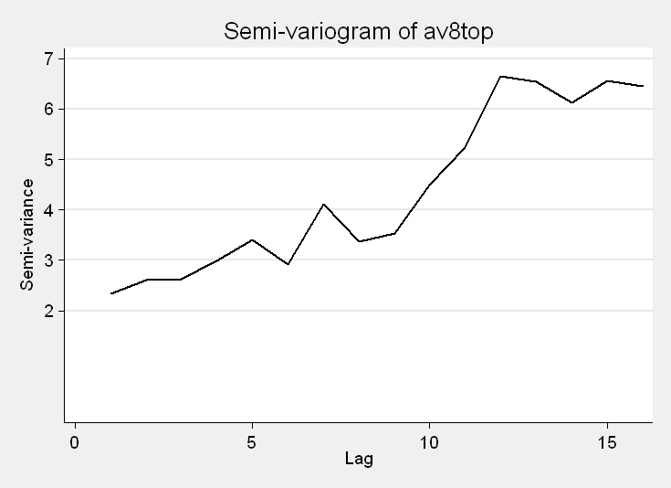
For the sake of an example, let’s imagine that instead of specific latitude and longitude locations, the stations are evenly spaced along a single latitude. If we assume the observations are in the order in which the stations appear, we can use the variog command. In the command, we indicate the measured outcome and we will opt for the calculated values to be listed. By default, a plot of the semi-variogram will be generated.
variog av8top, list
  +----------------------------------+
  | Lag   Semi-variance   # of pairs |
  |----------------------------------|
  |   1        2.328506           31 |
  |   2        2.615086           30 |
  |   3        2.629862           29 |
  |   4        2.983584           28 |
  |   5        3.415026           27 |
  |----------------------------------|
  |   6        2.923007           26 |
  |   7        4.104437           25 |
  |   8        3.378503           24 |
  |   9        3.531528           23 |
  |  10         4.49281           22 |
  |----------------------------------|
  |  11         5.22965           21 |
  |  12        6.657857           20 |
  |  13          6.5462           19 |
  |  14        6.126221           18 |
  |  15        6.556983           17 |
  |----------------------------------|
  |  16        6.451519           16 |
  +----------------------------------+
Next, let’s generate a variogram using the latitude and longitude of the stations. For this, we will use the variog2 command. While the lag distance in variog was assumed to be the distance between each evenly spaced observation, variog2 requires the user to specify the lag distance. Let’s look at a summary of our coordinates to get a sense of the distances existing in our data.
summarize lat lon

    Variable |       Obs        Mean    Std. Dev.       Min        Max
-------------+--------------------------------------------------------
         lat |        32     34.0146    .2228168    33.6275   34.69012
         lon |        32   -117.7078    .5683853  -118.5347  -116.2339
Based on this, we can calculate the maximum possible distance we might see in our data.
dis sqrt((33.6275 - 34.69012)^2 + (-118.5347 - -116.2339)^2)

2.5343326
As a starting point, we can choose a lag distance of .1 and we can examine distances up to 12 lags apart. We want to choose a lag distance that yields enough pairs in each lag to generate a variance that we trust. We might aim to have at least 15 pairs in each lag.
variog2 av8top lat lon, width(.1) lags(12) list


  +----------------------------------+
  | Lag   Semi-variance   # of pairs |
  |----------------------------------|
  |   1        4.729442            6 |
  |   2       1.8984963           31 |
  |   3       1.3789778           41 |
  |   4       2.7462469           50 |
  |   5       4.3899238           49 |
  |----------------------------------|
  |   6       4.1974818           43 |
  |   7       5.2652506           48 |
  |   8       7.3351494           41 |
  |   9       6.8823236           36 |
  |  10       8.0089961           29 |
  |----------------------------------|
  |  11       6.6957223           29 |
  |  12       7.1360346           23 |
  +----------------------------------+
We can see that our first lag contains only 6 pairs. We might increase the size of our lags and look at fewer of them.
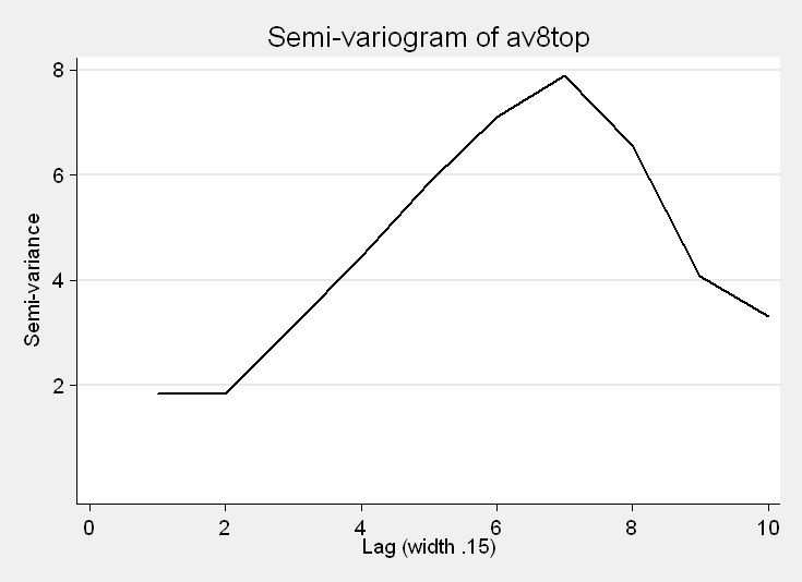
variog2  av8top lat lon, width(.15) lags(10) list

  +----------------------------------+
  | Lag   Semi-variance   # of pairs |
  |----------------------------------|
  |   1       1.8485044           21 |
  |   2       1.8412199           57 |
  |   3       3.1204523           74 |
  |   4       4.4411303           68 |
  |   5       5.8693088           70 |
  |----------------------------------|
  |   6       7.0979125           55 |
  |   7       7.8960334           44 |
  |   8       6.5713557           37 |
  |   9       4.0710902           23 |
  |  10       3.3176015           16 |
  +----------------------------------+
In the output, we can see lag distances up to 10*.15 = 1.5, the number of pairs that are this far apart in the dataset, and the semi-variance. As we can see from the plot, the semi-variance increases until the lag distance exceeds .15*7 = 1.05.
References:
- Cressie, Noel. Statistics for Spatial Data. John Wiley & Sons, Inc.: New York, 1991.
