Say that we use the hsb2 data file for the examples shown here.
use https://stats.idre.ucla.edu/stat/stata/notes/hsb2, clear
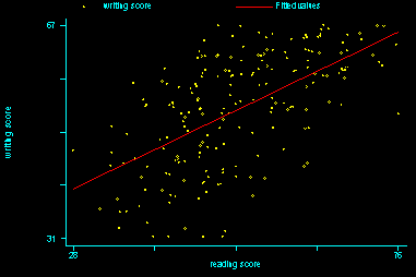
and say that you wanted to see the scatterplot and regression line between write and read. In Stata version 7 you might have done something like this.
regress write read
predict yhat
graph write yhat read, twoway symbol(oi) connect(.l) jitter(2) sort
And you would get a graph that looks something like this.
But if you execute the graph command in Stata version 8 or later you get this error message.
writegraph_g.new yhat read, twoway symbol(oi) connect(.l) jitter(2)
sort: class member function not found
write is not a valid graph subcommand
r(198);
You get this error message because the syntax of the graph command has been completely revised (and substantially enhanced) since version 8 and the syntax that you would have used in version 7 is not compatible with the current syntax.
There are two ways that you can deal with this. You can instruct Stata to run the command as though you were using Stata version 7 (instead of a later version) or you can convert the command to use the newer syntax. We discuss both below.
Using Stata 7 graphic commands in Stata 8
With a little bit of extra effort you can get Stata to run commands in the same way that they ran in Stata 7. With respect to graph commands, there are 3 strategies you could choose. The first is that you could use the graph7 command (abbreviation gr7 ) as shown below.
graph7 write yhat read, twoway symbol(oi) connect(.l) jitter(2) sort
and this produces a graph that looks just like you were using Stata version 7. Another trick is to use the version command to instruct Stata to run the graph command as though you were using version 7, as shown below.
version 7: graph write yhat read, twoway symbol(oi) connect(.l) jitter(2) sort
and again this produces a graph that looks just like you were using Stata version 7. If you are going to run a series of graph commands, you can issue a version 7 command on its own line and then all subsequent commands (graph commands and other types of commands) run as though they were from Stata version 7. This continues until you quit Stata or issue another version command on its own line. This is illustrated below.
version 7
graph write yhat read, twoway symbol(oi) connect(.l) jitter(2) sort
graph write
graph read
version 8 /* or 9 or 10 */
The strategy you choose will depend on the situation. These strategies work the same way in the Stata command window or in a Stata .do file.
Coverting Stata 7 graphics commands to the newer Stata syntax
You may want to just go ahead and convert your Stata 7 graphics commands to get the presentation quality graphs of the newer versions of Stata.
It is not possible to cover all of the different ways in which the current Stata graphics commands differ from the Stata 7 commands. The current Stata graph command includes six different graph types:
graph twoway              scatterplots, line plots, etc.
graph matrix              scatterplot matrices
graph bar                 bar charts
graph dot                 dot charts
graph box                 box and whisker plots
graph pie                 pie charts
The graph twoway type includes the following graphs among others:
scatter         scatterplot
line            line plot
connected       connected-line plot
area            line plot with shading
spike           spike plot
dot             dot plot
lowess          LOWESS line plot
lfit            linear prediction plot
qfit            quadratic prediction plot
lfitci          linear prediction plot with CIs
qfitci          quadratic prediction plot with CIs
function        line plot of function
histogram       histogram plot
kdensity        kernel density plot
Thus, a scatterplot can be done three different ways:
graph twoway scatter write read

twoway scatter write read

scatter write read
However, if you want to combine several twoway graphs in one plot, you will need to include the twoway type declaration. The following are examples of ways that you can produce the scatterplot and regression line that we tried in Stata 7 above.
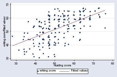
graph twoway (scatter write read, jitter(2)) (lfit write read, sort )

twoway (scatter write read, jitter(2)) (lfit write read, sort )

graph twoway scatter write read, jitter(2) || lfit write read, sort

twoway scatter write read, jitter(2) || lfit write read, sort
All of these constructions produce a graph that looks like this.
Note this will not work:
(scatter write read) (lfit write read)
Note: The separate plots indicated by enclosing the specific command in parentheses “()” or by separating the commands with two vertical bars “||”.
Problems converting symbol and connect options
Many Stata 7 twoway plots fail in the current version of Stata because Stata changed the way the symbol and connect options are implemented. In Stata 7 a scatter plot that includes two connected lines would be written like this:
graph write yhat read, twoway symbol(oi) connect(.l) jitter(2) sort
Note that, in both, symbol and connect the list of indicators is given without spaces. In newer versions of Stata you need to include a space between each of the items in the list. Further, you should change the option symbol to msymbol (for marker symbol). The equivalent Stata 8 or later command will look like this:
scatter write yhat read, msymbol(o i) connect(. l) jitter(2) sort
The above comments cover only a few of the many ways in which the current version of Stata graphics differ from the Stata 7 version. It is well worth you time to sit down and read the Stata Online Graphics Manual.


