Graphing results from the margins command can help in the interpretation of your model. Almost all of the needed results will be found in various matrices saved by margins. If you do not use the post option the matrices of interest are r(b) which has the point estimates, r(V) the variance-covariance matrix (standard errors are squares roots of the diagonal values), and r(at) which has the values used in the at option. If you do use the post option then the relevant matrices are e(b), e(V) and e(at).
Generally, the point estimates will be plotted on the y-axis. The x-axis will either be the at values or levels of a categorical predictor. The general strategy shown here will show how to get the necessary values for graphing into a Stata matrix which we will then save to data in memory using the svmat command. Once the values are part of the data we can plot the points using standard graph commands.
Example 1
Let’s start with a model that has a categorical by categorical interaction along with two continuous covariates. We will run the model as an anova but we would get the same results if we ran it as a regression.
use https://stats.idre.ucla.edu/stat/data/hsbdemo, clear

anova write prog##female math read

                           Number of obs =     200     R-squared     =  0.6932
                           Root MSE      = 6.59748     Adj R-squared =  0.5155

                  Source |  Partial SS    df       MS           F     Prob > F
             ------------+----------------------------------------------------
                   Model |   12394.507    73  169.787767       3.90     0.0000
                         |
                    prog |  22.3772184     2  11.1886092       0.26     0.7737
                  female |  1125.44586     1  1125.44586      25.86     0.0000
             prog#female |   287.95987     2  143.979935       3.31     0.0398
                    math |  2449.19165    39   62.799786       1.44     0.0670
                    read |  2015.49976    29  69.4999916       1.60     0.0411
                         |
                Residual |  5484.36799   126  43.5267301
             ------------+----------------------------------------------------
                   Total |   17878.875   199   89.843593
Next, we run the margins command to get the six adjust cell means from the 2 by 3 interaction. These adjusted cells means are called lsmeans in SAS or estimated marginal means in SPSS. After the margins command we will list the r(b) matrix.
margins prog#female, asbalanced

Adjusted predictions                              Number of obs   =        200

Expression   : Linear prediction, predict()
at           : prog             (asbalanced)
               female           (asbalanced)
               math             (asbalanced)
               read             (asbalanced)

------------------------------------------------------------------------------
             |            Delta-method
             |     Margin   Std. Err.      z    P>|z|     [95% Conf. Interval]
-------------+----------------------------------------------------------------
 prog#female |
        1 0  |   50.43791   1.969439    25.61   0.000     46.57788    54.29794
        1 1  |    56.9152   1.948113    29.22   0.000     53.09697    60.73343
        2 0  |   52.58387   1.408514    37.33   0.000     49.82323    55.34451
        2 1  |   55.05205    1.41875    38.80   0.000     52.27136    57.83275
        3 0  |   47.81982   2.108078    22.68   0.000     43.68806    51.95158
        3 1  |   57.29057   1.785628    32.08   0.000     53.79081    60.79034
------------------------------------------------------------------------------

matrix list r(b)

r(b)[1,6]
       1.prog#    1.prog#    2.prog#    2.prog#    3.prog#    3.prog#
     0.female   1.female   0.female   1.female   0.female   1.female
r1  50.437911    56.9152  52.583868  55.052054   47.81982  57.290573
Note that r(b) is a 1×6 matrix. We will want the 6×1 transpose of r(b) which we will call b.
matrix b=r(b)'

matrix list b

b[6,1]
                 r1
  1.prog#
0.female  50.437911
  1.prog#
1.female    56.9152
  2.prog#
0.female  52.583868
  2.prog#
1.female  55.052054
  3.prog#
0.female   47.81982
  3.prog#
1.female  57.290573
If you look back at the margins output you will see a column for prog that has two 1’s followed by two 2’s and then two 3’s. We will create this array using a Kronecker product of a column vector (123) and a column vector (11).
matrix prg=(123)#(11)  /* # is the kronecker product operator */

matrix list prg

prg[6,1]
        c1:
        c1
r1:r1    1
r1:r2    1
r2:r3    2
r2:r4    2
r3:r5    3
r3:r6    3
We will use this same trick again to create an series of alternating 0’s and 1’s. Next, we will combine the three columns together into a matrix called c.
matrix fem=(111)#(01)  /* # is the kronecker product operator */

matrix list fem

fem[6,1]
        c1:
        c1
r1:r1    0
r1:r2    1
r2:r3    0
r2:r4    1
r3:r5    0
r3:r6    1

matrix c=prg,fem,b

matrix list c

c[6,3]
              c1:        c1:
              c1         c1         r1
r1:r1          1          0  50.437911
r1:r2          1          1    56.9152
r2:r3          2          0  52.583868
r2:r4          2          1  55.052054
r3:r5          3          0   47.81982
r3:r6          3          1  57.290573
Now we can save c to data using the svmat command.
svmat c, names(c)

clist c1-c3 in 1/7

            c1         c2         c3
  1.         1          0   50.43791
  2.         1          1    56.9152
  3.         2          0   52.58387
  4.         2          1   55.05206
  5.         3          0   47.81982
  6.         3          1   57.29057
  7.         .          .          .
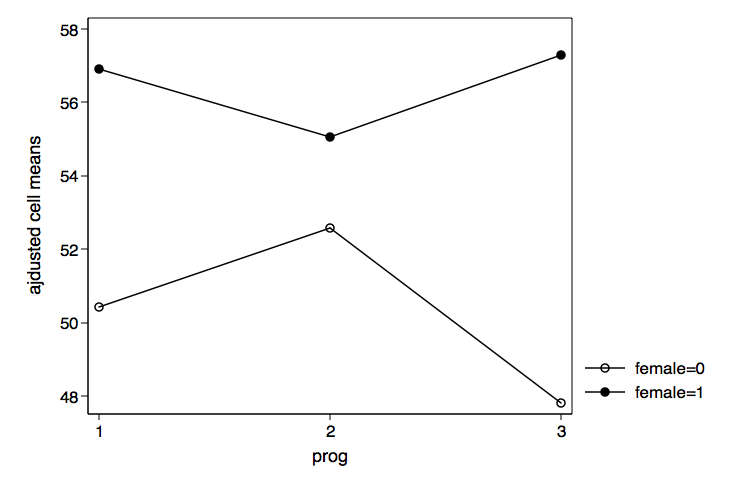
We can now plot the adjusted cell means for prog by female using graph twoway
/* plot prog by female */
graph twoway (connect c3 c1 if c2==0)(connect c3 c1 if c2==1), ///
             xlabel(1 2 3) legend(order(1 "female=0" 2 "female=1")) ///
             xtitle(prog) ytitle(ajdusted cell means) ///
             name(prog_by_female, replace)
We can also graph the results for female by prog just by reversing c1 and c2 in the graph twoway command.
/* plot female by prog */
graph twoway (connect c3 c2 if c1==1)(connect c3 c2 if c1==2) ///
             (connect c3 c2 if c1==3), xlabel(0 1) ///
             legend(order(1 "prog=1" 2 "prog=2" 3 "prog=3")) ///
             xtitle(female) ytitle(ajdusted cell means) ///
             name(female_by_prog, replace)

Example 2
For our second example we will graph the results of a categorical by continuous interaction from a logistic regression model.
use https://stats.idre.ucla.edu/stat/data/logitcatcon, clear

logit y i.f##c.s, nolog

Logistic regression                               Number of obs   =        200
                                                  LR chi2(3)      =      71.01
                                                  Prob > chi2     =     0.0000
Log likelihood =  -96.28586                       Pseudo R2       =     0.2694

------------------------------------------------------------------------------
           y |      Coef.   Std. Err.      z    P>|z|     [95% Conf. Interval]
-------------+----------------------------------------------------------------
         1.f |   5.786811   2.302518     2.51   0.012     1.273959    10.29966
           s |   .1773383   .0364362     4.87   0.000     .1059248    .2487519
             |
       f#c.s |
          1  |  -.0895522   .0439158    -2.04   0.041    -.1756255   -.0034789
             |
       _cons |  -9.253801    1.94189    -4.77   0.000    -13.05983   -5.447767
------------------------------------------------------------------------------
We will use the margins command to get the predicted probabilites for 11 values of s from 20 to 70 for both f equal zero and f equal one. The vsquish option just reduces the number of blank lines in the output.
margins f, at(s=(20(5)70)) vsquish

Adjusted predictions                              Number of obs   =        200
Model VCE    : OIM

Expression   : Pr(y), predict()
1._at        : s               =          20
2._at        : s               =          25
3._at        : s               =          30
4._at        : s               =          35
5._at        : s               =          40
6._at        : s               =          45
7._at        : s               =          50
8._at        : s               =          55
9._at        : s               =          60
10._at       : s               =          65
11._at       : s               =          70

------------------------------------------------------------------------------
             |            Delta-method
             |     Margin   Std. Err.      z    P>|z|     [95% Conf. Interval]
-------------+----------------------------------------------------------------
       _at#f |
        1 0  |   .0033115   .0040428     0.82   0.413    -.0046123    .0112353
        1 1  |   .1529993    .098668     1.55   0.121    -.0403864    .3463851
        2 0  |   .0079995   .0083179     0.96   0.336    -.0083033    .0243023
        2 1  |   .2188574   .1104097     1.98   0.047     .0024583    .4352564
        3 0  |   .0191964   .0164503     1.17   0.243    -.0130456    .0514383
        3 1  |   .3029251   .1126363     2.69   0.007      .082162    .5236882
        4 0  |   .0453489   .0304422     1.49   0.136    -.0143166    .1050145
        4 1  |   .4026401   .1026147     3.92   0.000      .201519    .6037612
        5 0  |   .1033756   .0500784     2.06   0.039     .0052238    .2015275
        5 1  |   .5111116   .0827069     6.18   0.000      .349009    .6732142
        6 0  |   .2186457   .0674192     3.24   0.001     .0865065    .3507849
        6 1  |   .6185467   .0611384    10.12   0.000     .4987176    .7383758
        7 0  |   .4044675   .0706157     5.73   0.000     .2660634    .5428717
        7 1  |   .7155135   .0476424    15.02   0.000     .6221361    .8088909
        8 0  |    .622414   .0675171     9.22   0.000     .4900828    .7547452
        8 1  |    .795962   .0437198    18.21   0.000     .7102727    .8816513
        9 0  |   .8000327   .0610245    13.11   0.000     .6804269    .9196385
        9 1  |   .8581703   .0421992    20.34   0.000     .7754613    .9408793
       10 0  |   .9066322   .0443791    20.43   0.000     .8196508    .9936136
       10 1  |   .9037067   .0387213    23.34   0.000     .8278143    .9795991
       11 0  |   .9592963   .0267857    35.81   0.000     .9067973    1.011795
       11 1  |   .9357181   .0332641    28.13   0.000     .8705218    1.000914
------------------------------------------------------------------------------
In total, there are 22 values in the r(b) matrix. Once again we will put these values into a matrix called b.
matrix b=r(b)'

matrix list b

b[22,1]
                   r1
 1._at#0.f  .00331151
 1._at#1.f  .15299932
 2._at#0.f  .00799952
 2._at#1.f  .21885736
 3._at#0.f  .01919637
 3._at#1.f  .30292513
 4._at#0.f  .04534893
 4._at#1.f   .4026401
 5._at#0.f  .10337563
 5._at#1.f  .51111162
 6._at#0.f  .21864569
 6._at#1.f   .6185467
 7._at#0.f  .40446752
 7._at#1.f  .71551351
 8._at#0.f    .622414
 8._at#1.f  .79596199
 9._at#0.f   .8000327
 9._at#1.f  .85817031
10._at#0.f   .9066322
10._at#1.f   .9037067
11._at#0.f  .95929634
11._at#1.f  .93571812
Next, we need the 11 values of read found in the r(at) matrix. However, r(at) is an 11×3 matrix for which we only need the column labeled s. We also need to have two of each of the values of read which we will get by again using the Kronecker product.
matrix at=r(at)

matrix list at

at[11,3]
      0b.   1.
       f    f    s
 r1    .    .   20
 r2    .    .   25
 r3    .    .   30
 r4    .    .   35
 r5    .    .   40
 r6    .    .   45
 r7    .    .   50
 r8    .    .   55
 r9    .    .   60
r10    .    .   65
r11    .    .   70

matrix at=at[1...,"s"]#(11)  /* # is the kronecker operator */

matrix list at

at[22,1]
          s:
         c1
  r1:r1  20
  r1:r2  20
  r2:r3  25
  r2:r4  25
  r3:r5  30
  r3:r6  30
  r4:r7  35
  r4:r8  35
  r5:r9  40
 r5:r10  40
 r6:r11  45
 r6:r12  45
 r7:r13  50
 r7:r14  50
 r8:r15  55
 r8:r16  55
 r9:r17  60
 r9:r18  60
r10:r19  65
r10:r20  65
r11:r21  70
r11:r22  70
We will put the at and b matrices together into matrix p and save the values to data. In this case it is easier to create the alternating series of 0’s and 1’s once the data are in memory using the line number modulo 2 with the not prefix so that the series starts with zero.
matrix p=at,b

matrix list p

p[22,2]
                 s:
                c1         r1
  r1:r1         20  .00331151
  r1:r2         20  .15299932
  r2:r3         25  .00799952
  r2:r4         25  .21885736
  r3:r5         30  .01919637
  r3:r6         30  .30292513
  r4:r7         35  .04534893
  r4:r8         35   .4026401
  r5:r9         40  .10337563
 r5:r10         40  .51111162
 r6:r11         45  .21864569
 r6:r12         45   .6185467
 r7:r13         50  .40446752
 r7:r14         50  .71551351
 r8:r15         55    .622414
 r8:r16         55  .79596199
 r9:r17         60   .8000327
 r9:r18         60  .85817031
r10:r19         65   .9066322
r10:r20         65   .9037067
r11:r21         70  .95929634
r11:r22         70  .93571812

svmat p, names(p)

generate p3 = ~mod(_n,2) in 1/22

clist p1-p3 in 1/23


            p1         p2         p3
  1.        20   .0033115          0
  2.        20   .1529993          1
  3.        25   .0079995          0
  4.        25   .2188574          1
  5.        30   .0191964          0
  6.        30   .3029251          1
  7.        35   .0453489          0
  8.        35   .4026401          1
  9.        40   .1033756          0
 10.        40   .5111116          1
 11.        45   .2186457          0
 12.        45   .6185467          1
 13.        50   .4044675          0
 14.        50   .7155135          1
 15.        55    .622414          0
 16.        55    .795962          1
 17.        60   .8000327          0
 18.        60   .8581703          1
 19.        65   .9066322          0
 20.        65   .9037067          1
 21.        70   .9592963          0
 22.        70   .9357181          1
 23.         .          .          .
Now we can go ahead and graph the probabilities for f equal zero and f equal one using the graph twoway command.
graph twoway (line p2 p1 if p3==0)(line p2 p1 if p3==1), ///
      legend(order(1 "f=0" 2 "f=1")) xtitle(variable s) ///
      ytitle(probability) name(probability, replace)
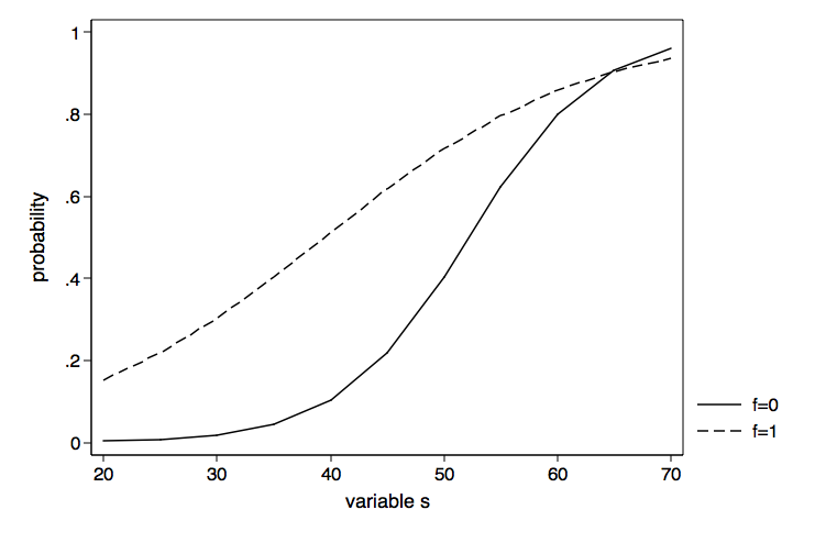
The graph of the probabilities above is nice as far as it goes but the presentation of the results might be clearer if we were to graph the difference in probabilities between f equal zero and f equal one. To do this we will need to rerun the margins command computing the discrete change for f at each value of read. We can get the difference using the dydx (derivative) option.
margins, dydx(f) at(s=(20(5)70)) vsquish

Conditional marginal effects                      Number of obs   =        200
Model VCE    : OIM

Expression   : Pr(y), predict()
dy/dx w.r.t. : 1.f
1._at        : s               =          20
2._at        : s               =          25
3._at        : s               =          30
4._at        : s               =          35
5._at        : s               =          40
6._at        : s               =          45
7._at        : s               =          50
8._at        : s               =          55
9._at        : s               =          60
10._at       : s               =          65
11._at       : s               =          70

------------------------------------------------------------------------------
             |            Delta-method
             |      dy/dx   Std. Err.      z    P>|z|     [95% Conf. Interval]
-------------+----------------------------------------------------------------
1.f          |
         _at |
          1  |   .1496878   .0987508     1.52   0.130    -.0438602    .3432358
          2  |   .2108578   .1107226     1.90   0.057    -.0061545    .4278701
          3  |   .2837288   .1138312     2.49   0.013     .0606236    .5068339
          4  |   .3572912    .107035     3.34   0.001     .1475064     .567076
          5  |    .407736   .0966865     4.22   0.000     .2182339     .597238
          6  |    .399901   .0910124     4.39   0.000       .22152     .578282
          7  |    .311046   .0851843     3.65   0.000     .1440878    .4780042
          8  |    .173548   .0804362     2.16   0.031     .0158959    .3312001
          9  |   .0581376   .0741941     0.78   0.433    -.0872801    .2035553
         10  |  -.0029255   .0588969    -0.05   0.960    -.1183612    .1125102
         11  |  -.0235782    .042708    -0.55   0.581    -.1072843    .0601279
------------------------------------------------------------------------------
Note: dy/dx for factor levels is the discrete change from the base level.
Once again we will need the r(b) and r(at) values. But, we need to be careful this time because of the way that margins parameterizes these estimates there are 11 zero’s in the r(b) matrix before the 11 point estimates of interest. We will need to drop all of the rows with zero values.
matrix b=r(b)'

matrix list b

b[22,1]
                     r1
 0b.f:1._at           0
 0b.f:2._at           0
 0b.f:3._at           0
 0b.f:4._at           0
 0b.f:5._at           0
 0b.f:6._at           0
 0b.f:7._at           0
 0b.f:8._at           0
 0b.f:9._at           0
0b.f:10._at           0
0b.f:11._at           0
  1.f:1._at   .14968781
  1.f:2._at   .21085784
  1.f:3._at   .28372876
  1.f:4._at   .35729117
  1.f:5._at   .40773598
  1.f:6._at     .399901
  1.f:7._at   .31104599
  1.f:8._at   .17354799
  1.f:9._at   .05813761
 1.f:10._at  -.00292551
 1.f:11._at  -.02357822

matrix b=b[12...,1]

matrix list b

b[11,1]
                    r1
 1.f:1._at   .14968781
 1.f:2._at   .21085784
 1.f:3._at   .28372876
 1.f:4._at   .35729117
 1.f:5._at   .40773598
 1.f:6._at     .399901
 1.f:7._at   .31104599
 1.f:8._at   .17354799
 1.f:9._at   .05813761
1.f:10._at  -.00292551
1.f:11._at  -.02357822

matrix at=r(at)

matrix at=at[1...,"s"]

matrix list at

at[11,1]
      s
 r1  20
 r2  25
 r3  30
 r4  35
 r5  40
 r6  45
 r7  50
 r8  55
 r9  60
r10  65
r11  70
For this graph of the differences in probabilities we will also include the lines for the 95% confidence interval. We will need to compute the upper and lower confidence values manually. To do this we will need the standard errors from the margins command. We will begin by getting the variance-covariance matrix of the estimates. Once again we will have to drop all of the rows and columns that are all zeros.
matrix v=r(V)

matrix v=v[12...,12...]

matrix list v

symmetric v[11,11]
                   1.f:        1.f:        1.f:        1.f:        1.f:        1.f:        1.f:        1.f:
                     1.          2.          3.          4.          5.          6.          7.          8.
                   _at         _at         _at         _at         _at         _at         _at         _at
 1.f:1._at   .00975172
 1.f:2._at   .01090899   .01225949
 1.f:3._at   .01106858   .01252966   .01295755
 1.f:4._at   .00988489   .01133267   .01196523    .0114565
 1.f:5._at   .00746032   .00876206   .00961621   .00982147   .00934828
 1.f:6._at   .00437948   .00540815   .00638981   .00727808   .00804735   .00828325
 1.f:7._at   .00138994   .00201386   .00284747    .0039552    .0053869   .00685686   .00725637
 1.f:8._at  -.00090133  -.00072541  -.00028361   .00050889   .00177443   .00364155   .00568431   .00646999
 1.f:9._at  -.00219008  -.00231219  -.00218045  -.00173163  -.00085595   .00078305    .0033247   .00541876
1.f:10._at  -.00260473  -.00282965  -.00279956  -.00246344  -.00177185  -.00047237   .00167411   .00372089
1.f:11._at  -.00249143  -.00271383  -.00268483  -.00235557  -.00172561  -.00069732   .00085579   .00235456

                   1.f:        1.f:        1.f:
                     9.         10.         11.
                   _at         _at         _at
 1.f:9._at   .00550476
1.f:10._at   .00422715   .00346884
1.f:11._at   .00284913   .00245636   .00182397
The standard errors are found by taking the square roots of the digonal values of v. This actually invloves a series of steps; getting the diagonal values (vecdiag), putting them into a diagonal matrix (diag), getting the square roots (cholesky) and finally putting the values into a column vector (vecdiag). The one step that may not have been obvious is using the Cholesky decompostion on a diagonal matrix which gives us the square roots of the diagonal values. These four matrix functions are included in a single command shown below.
matrix se=vecdiag(cholesky(diag(vecdiag(v))))'

matrix list se

se[11,1]
                   r1
 1.f:1._at  .09875081
 1.f:2._at   .1107226
 1.f:3._at  .11383123
 1.f:4._at  .10703502
 1.f:5._at   .0966865
 1.f:6._at  .09101237
 1.f:7._at  .08518432
 1.f:8._at  .08043624
 1.f:9._at  .07419408
1.f:10._at  .05889686
1.f:11._at  .04270799
Next, we will put the at, b and se matrices together into matrix d and save them to the data in memory. Now we can generate the values for the upper and lower 95% confidence intervals.
matrix d=at,b,se

matrix list d

d[11,3]
              s          r1          r1
 r1          20   .14968781   .09875081
 r2          25   .21085784    .1107226
 r3          30   .28372876   .11383123
 r4          35   .35729117   .10703502
 r5          40   .40773598    .0966865
 r6          45     .399901   .09101237
 r7          50   .31104599   .08518432
 r8          55   .17354799   .08043624
 r9          60   .05813761   .07419408
r10          65  -.00292551   .05889686
r11          70  -.02357822   .04270799

svmat d, names(d)
generate ul = d2 + 1.96*d3
generate ll = d2 - 1.96*d3

clist d1-ll in 1/12

            d1         d2         d3         ul         ll
  1.        20   .1496878   .0987508   .3432394  -.0438638
  2.        25   .2108578   .1107226   .4278741  -.0061585
  3.        30   .2837287   .1138312    .506838   .0606195
  4.        35   .3572912    .107035   .5670798   .1475025
  5.        40    .407736   .0966865   .5972415   .2182304
  6.        45    .399901   .0910124   .5782852   .2215168
  7.        50    .311046   .0851843   .4780073   .1440847
  8.        55    .173548   .0804362    .331203    .015893
  9.        60   .0581376   .0741941    .203558  -.0872828
 10.        65  -.0029255   .0588969   .1125123  -.1183634
 11.        70  -.0235782    .042708   .0601294  -.1072859
 12.         .          .          .          .          .
Here is the graph twoway command to plot the differeces in probability with lines for the upper and lower confidence intervals.
graph twoway (line d2 ul ll d1), yline(0) legend(off) ///
       xtitle(variable s) ytitle(difference in probability) ///
       name(difference1, replace)
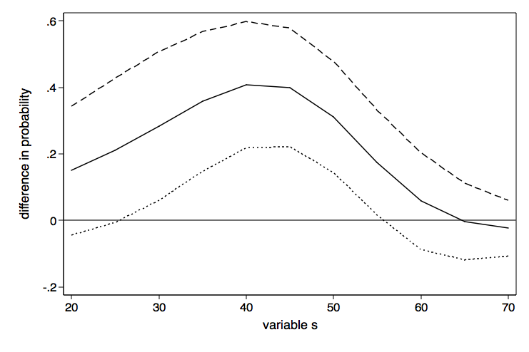
As nice as the above graph is, it might look better done as a range plot with area shading between the upper and lower confidence bounds.
graph twoway (rarea ul ll d1, color(gs13) lcolor(gs13)) ///
             (line d2 d1), yline(0) legend(off) ///
             xtitle(variable s) ytitle(difference in probability) ///
             name(difference2, replace)
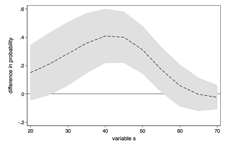
If you want the lines in these graphs to be smoother, just include more values in the at option, say (20(2)70) instead of (20(5)70).
Below you will find all of the code from both examples without the commentary.
/* example 1 --  plot adjusted cell means */

use https://stats.idre.ucla.edu/stat/data/hsbdemo, clear
anova write prog##female math read

margins prog#female, asbalanced
mat b=r(b)'
mat prg=(123)#(11)
mat fem=(111)#(01)
mat c=prg,fem,b
svmat c, names(c)

/* plot prog by female */
graph twoway (connect c3 c1 if c2==0)(connect c3 c1 if c2==1), ///
       xlabel(1 2 3) legend(order(1 "female=0" 2 "female=1")) ///
       xtitle(prog) ytitle(ajdusted cell means) ///
       name(prog_by_female, replace)

/* plot female by prog */
graph twoway (connect c3 c2 if c1==1)(connect c3 c2 if c1==2)(connect c3 c2 if c1==3), ///
       xlabel(0 1) legend(order(1 "prog=1" 2 "prog=2" 3 "prog=3")) ///
       xtitle(female) ytitle(ajdusted cell means) ///
       name(female_by_prog, replace)


/* example 2 -- categorical by continuous */

use https://stats.idre.ucla.edu/stat/data/logitcatcon, clear
logit y i.f##c.s, nolog

/* plot probabilities by categorical variable */
margins f, at(s=(20(5)70)) vsquish
mat b=r(b)'
mat at=r(at)
mat at=at[1...,3]#(11)
mat p=at,b
svmat p, names(p)
generate p3 = ~mod(_n,2) in 1/52
graph twoway (line p2 p1 if p3==0)(line p2 p1 if p3==1), ///
       legend(order(1 "f=0" 2 "f=1")) xtitle(variable s) ///
       ytitle(probability) name(probability, replace)


/* difference in probabilities */
margins, dydx(f) at(s=(20(5)70)) vsquish
mat b=r(b)'
mat at=r(at)
mat at=at[1...,3]
local nrow=rowsof(at)
mat b=b[`nrow'+1...,1]
mat se=r(V)
mat se=se[`nrow'+1...,`nrow'+1...]
mat se=vecdiag(cholesky(diag(vecdiag(se))))'
mat d=at,b,se
mat lis d
svmat d, names(d)
gen ul = d2 + 1.96*d3
gen ll = d2 - 1.96*d3
graph twoway (line d2 ul ll d1), yline(0) legend(off) ///
       xtitle(variable s) ytitle(difference in probability) ///
       name(difference1, replace)

graph twoway (rarea ul ll d1, color(gs13) lcolor(gs13)) ///
       (line d2 d1), yline(0) legend(off) ///
       xtitle(variable s) ytitle(difference in probability) ///
       name(difference2, replace)