This page is Part 2 of a two-page sequence. If you have reached here without reading the first part you should go back because there is a lot of explanitory material that is not covered on this page. Go back now.
This page presents an approach for testing two-way interactions at each level of a third variable and for doing tests of simple main-effects on two-way interactions without having to copy the sums of squares and degrees of freedom and computing F-ratios manually.
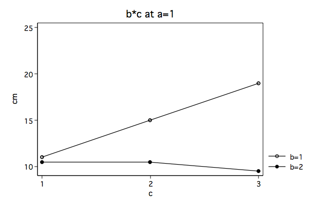
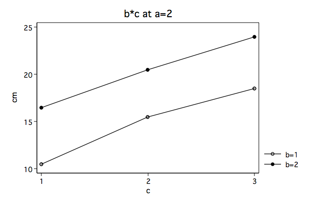
As a review from the previous page we will look at the full three-factor anova along with the plots of the b*c interactions separately for a==1 and a==2.
use https://stats.idre.ucla.edu/stat/stata/faq/threeway, clear

anova y a b c a*b a*c b*c a*b*c

                          Number of obs =      24     R-squared     =  0.9689
                           Root MSE      =  1.1547     Adj R-squared =  0.9403

                  Source |  Partial SS    df       MS           F     Prob > F
              -----------+----------------------------------------------------
                   Model |  497.833333    11  45.2575758      33.94     0.0000
                         |
                       a |         150     1         150     112.50     0.0000
                       b |  .666666667     1  .666666667       0.50     0.4930
                       c |  127.583333     2  63.7916667      47.84     0.0000
                     a*b |  160.166667     1  160.166667     120.13     0.0000
                     a*c |       18.25     2       9.125       6.84     0.0104
                     b*c |  22.5833333     2  11.2916667       8.47     0.0051
                   a*b*c |  18.5833333     2  9.29166667       6.97     0.0098
                         |
                Residual |          16    12  1.33333333
              -----------+----------------------------------------------------
                   Total |  513.833333    23  22.3405797


Again, we note that the b*c interaction looks very different at a==1 then at a==2.
Before we get into the alternative method of explaining the three-way interaction we will review effect-coding for variables b and c. In the table below, column (1) is the effect-coding for b main-effect; columns (2) and (4) are for the c main-effect; and columns (4) and (5) are for the b*c interaction.
      Effect Coding
    (1) (2) (3) (4) (5)
b c  b  c1  c2  bc1 bc2
1 1  1   1   0   1   0
1 2  1   0   1   0   1
1 3  1  -1  -1  -1  -1
2 1 -1   1   0  -1   0
2 2 -1   0   1   0  -1
2 3 -1  -1  -1   1   1
|
Next, we will run the anova model with b*c nested in a. You will note that the residual sums of squares and degrees of freedom are the same as for the original three factor model.
/* anova for b*c at levels of a */

anova y b c b*c|a

                           Number of obs =      24     R-squared     =  0.9689
                           Root MSE      =  1.1547     Adj R-squared =  0.9403

                  Source |  Partial SS    df       MS           F     Prob > F
              -----------+----------------------------------------------------
                   Model |  497.833333    11  45.2575758      33.94     0.0000
                         |
                       b |  .666666667     1  .666666667       0.50     0.4930
                       c |  127.583333     2  63.7916667      47.84     0.0000
                   b*c|a |  369.583333     8  46.1979167      34.65     0.0000
                         |
                Residual |          16    12  1.33333333
              -----------+----------------------------------------------------
                   Total |  513.833333    23  22.3405797
If we use the test command with the showorder option, we can see what each of the parameters are.
test, showorder

 Order of columns in the design matrix
      1: _cons
      2: (b==1)
      3: (b==2)
      4: (c==1)
      5: (c==2)
      6: (c==3)
      7: (b==1)*(c==1)*(a==1)
      8: (b==1)*(c==1)*(a==2)
      9: (b==1)*(c==2)*(a==1)
     10: (b==1)*(c==2)*(a==2)
     11: (b==1)*(c==3)*(a==1)
     12: (b==1)*(c==3)*(a==2)
     13: (b==2)*(c==1)*(a==1)
     14: (b==2)*(c==1)*(a==2)
     15: (b==2)*(c==2)*(a==1)
     16: (b==2)*(c==2)*(a==2)
     17: (b==2)*(c==3)*(a==1)
     18: (b==2)*(c==3)*(a==2)
From the table above we can see that the b*c interaction for each level of a are found in rows 7 through 18. We will use the effect-coding from columns (4) and (5) above aligned with the appropriate element of matrices bc1 and bc2 to test the interaction separately at each level of a. For example, the -1’s in column (4) are found when b==1 & c==1 and when b==2 & c==1. For the case when a==1 in the showorder these vales occur in row 11 and row 13. The matrices used with the test are created using the column to represent the parameter, so in the first row of bc1 columns 11 and 13 will have -1’s. The two rows of bc1 test the b*c interaction at a==1, while bc2 tests the interaction at a==2.
matrix bc1=(0,0,0,0,0,0,1,0,0,0,-1,0,-1,0,0,0,1,0 ///
            0,0,0,0,0,0,0,0,1,0,-1,0,0,0,-1,0,1,0)

matrix list bc1

bc1[2,18]
     c1   c2   c3   c4   c5   c6   c7   c8   c9  c10  c11  c12  c13  c14  c15  c16  c17  c18
r1    0    0    0    0    0    0    1    0    0    0   -1    0   -1    0    0    0    1    0
r2    0    0    0    0    0    0    0    0    1    0   -1    0    0    0   -1    0    1    0

matrix bc2=(0,0,0,0,0,0,0,1,0,0,0,-1,0,-1,0,0,0,1 ///
            0,0,0,0,0,0,0,0,0,1,0,-1,0,0,0,-1,0,1)

matrix list bc2

bc2[2,18]
     c1   c2   c3   c4   c5   c6   c7   c8   c9  c10  c11  c12  c13  c14  c15  c16  c17  c18
r1    0    0    0    0    0    0    0    1    0    0    0   -1    0   -1    0    0    0    1
r2    0    0    0    0    0    0    0    0    0    1    0   -1    0    0    0   -1    0    1
Next, using the test command with the test() option we test the interactions.
/* test b*c at a==1 */

test, test(bc1)

 ( 1)  b[1]*c[1]*a[1] - b[1]*c[3]*a[1] - b[2]*c[1]*a[1] + b[2]*c[3]*a[1] = 0
 ( 2)  b[1]*c[2]*a[1] - b[1]*c[3]*a[1] - b[2]*c[2]*a[1] + b[2]*c[3]*a[1] = 0

       F(  2,    12) =   15.25
            Prob > F =    0.0005

/* test b*c at a==2 */

test, test(bc2)

 ( 1)  b[1]*c[1]*a[2] - b[1]*c[3]*a[2] - b[2]*c[1]*a[2] + b[2]*c[3]*a[2] = 0
 ( 2)  b[1]*c[2]*a[2] - b[1]*c[3]*a[2] - b[2]*c[2]*a[2] + b[2]*c[3]*a[2] = 0

       F(  2,    12) =    0.19
            Prob > F =    0.8314

return list /* to see the F-ratio to more decimal places */

scalars:
                  r(p) =  .8314118892405968
                 r(df) =  2
                  r(F) =  .1874999999999936
               r(df_r) =  12
               r(drop) =  0
These are the same two F-ratios (15.25 and .1875) that we computed using the original method in Part 1. And, just as in Part 1, we need to use the appropriate critical values for the F-ratios and not just go by the printed p-values.
Now that we know that the b*c interaction at a==1 is sifnificant, we can move on to testing whether there are significant difference in the levels of c for each of the levels of b at a==1. To accomplish this we will run another anova model, this time looking a c nested in a*b. Once again, please note, that the residual SS and df are the same as the original three factor model.
/* anova for testing c holding a & b constant */

anova y c|a*b

                           Number of obs =      24     R-squared     =  0.9689
                           Root MSE      =  1.1547     Adj R-squared =  0.9403

                  Source |  Partial SS    df       MS           F     Prob > F
              -----------+----------------------------------------------------
                   Model |  497.833333    11  45.2575758      33.94     0.0000
                         |
                   c|a*b |  497.833333    11  45.2575758      33.94     0.0000
                         |
                Residual |          16    12  1.33333333
              -----------+----------------------------------------------------
                   Total |  513.833333    23  22.3405797
Let’s run test with the showorder option for this model.
test, showorder

 Order of columns in the design matrix
      1: _cons
      2: (c==1)*(a==1)*(b==1)
      3: (c==1)*(a==1)*(b==2)
      4: (c==1)*(a==2)*(b==1)
      5: (c==1)*(a==2)*(b==2)
      6: (c==2)*(a==1)*(b==1)
      7: (c==2)*(a==1)*(b==2)
      8: (c==2)*(a==2)*(b==1)
      9: (c==2)*(a==2)*(b==2)
     10: (c==3)*(a==1)*(b==1)
     11: (c==3)*(a==1)*(b==2)
     12: (c==3)*(a==2)*(b==1)
     13: (c==3)*(a==2)*(b==2)
Using the effect-coding columns (2) and (3) from above, we will create two more test matrices aligning the parameters with the c main-effect. This time there will only be 13 columns in each matrix.
matrix c1=(0,1,0,0,0,0,0,0,0,-1,0,0,0 ///
           0,0,0,0,0,1,0,0,0,-1,0,0,0)

matrix list c1

c1[2,13]
     c1   c2   c3   c4   c5   c6   c7   c8   c9  c10  c11  c12  c13
r1    0    1    0    0    0    0    0    0    0   -1    0    0    0
r2    0    0    0    0    0    1    0    0    0   -1    0    0    0

matrix c2=(0,0,1,0,0,0,0,0,0,0,-1,0,0 ///
           0,0,0,0,0,0,1,0,0,0,-1,0,0)

matrix list c2

c2[2,13]
     c1   c2   c3   c4   c5   c6   c7   c8   c9  c10  c11  c12  c13
r1    0    0    1    0    0    0    0    0    0    0   -1    0    0
r2    0    0    0    0    0    0    1    0    0    0   -1    0    0
We can now go to the test commands themselves.
/* test for c at a==1 & b==1 */

test, test(c1)

 ( 1)  c[1]*a[1]*b[1] - c[3]*a[1]*b[1] = 0
 ( 2)  c[2]*a[1]*b[1] - c[3]*a[1]*b[1] = 0

       F(  2,    12) =   24.00
            Prob > F =    0.0001

/* test for c at a==1 & b==2 */

test, test(c2)

 ( 1)  c[1]*a[1]*b[2] - c[3]*a[1]*b[2] = 0
 ( 2)  c[2]*a[1]*b[2] - c[3]*a[1]*b[2] = 0

       F(  2,    12) =    0.50
            Prob > F =    0.6186
Once again, these F-ratios (24.0 and 0.50) are the same as those computed using the method in Part 1. And, as in Part 1, we would have to finish up by running pair-wise comparisons among the means at a==1, b==1. We can run the same tukeyhsd command as we did before.
Just a word of warning. You won’t be able to cut-and-paste the Stata commands from this page, like the previous page, because it is unlikely that your model will follow the same patterns of levels and effects as this example. It will be necessary that you work out the correct coding for each research project individually.
References
Kirk, Roger E. (1995) Experimental Design: Procedures for the Behavioral Sciences, Third Edition. Monterey, California: Brooks/Cole Publishing.
