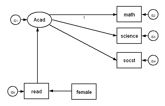
Below is the diagram of a simple structural equation model. The dependent variable is a latent variable Acad with three observed indicators, math, science and socst. There are two additional observed variables, the independent variable female and a mediator variable read. (Note, variables in squares are observed (manifest variables), those in circles are latent. The small circles with ε are error terms, i.e., residual variances).
We will analyze this model using the sem command with the hsbdemo dataset.
use https://stats.idre.ucla.edu/stat/data/hsbdemo, clear

sem (Acad->math science socst)(Acad<-read)(read<-female), ///
    mean(female) var(female)

Endogenous variables

Observed:     read
Measurement:  math science socst
Latent:       Acad

Exogenous variables

Observed:     female

Fitting target model:

Iteration 0:   log likelihood =  -6737.783  (not concave)
[output omitted]
Iteration 13:  log likelihood = -2949.3343

Structural equation model                       Number of obs      =       200
Estimation method  = ml
Log likelihood     = -2949.3343

 ( 1)  [math]Acad = 1
------------------------------------------------------------------------------
             |                 OIM
             |      Coef.   Std. Err.      z    P>|z|     [95% Conf. Interval]
-------------+----------------------------------------------------------------
Structural   |
  read <-    |
      female |  -1.090231   1.450201    -0.75   0.452    -3.932572     1.75211
       _cons |   52.82418   1.070598    49.34   0.000     50.72584    54.92251
  -----------+----------------------------------------------------------------
  Acad <-    |
        read |    .620298   .0461021    13.45   0.000     .5299395    .7106565
-------------+----------------------------------------------------------------
Measurement  |
  math <-    |
        Acad |          1  (constrained)
       _cons |   20.24684   2.456312     8.24   0.000     15.43255    25.06112
  -----------+----------------------------------------------------------------
  science <- |
        Acad |   .9874351   .0908878    10.86   0.000     .8092984    1.165572
       _cons |   19.85891   2.737663     7.25   0.000     14.49319    25.22463
  -----------+----------------------------------------------------------------
  socst <-   |
        Acad |   .9940776   .1030617     9.65   0.000     .7920804    1.196075
       _cons |   20.19871   3.181537     6.35   0.000     13.96301     26.4344
-------------+----------------------------------------------------------------
Mean         |
      female |       .545   .0352119    15.48   0.000      .475986     .614014
-------------+----------------------------------------------------------------
Variance     |
      e.math |   31.77659   4.630872                       23.8814    42.28192
   e.science |   43.37236   5.487556                      33.84678    55.57874
     e.socst |    59.7846   7.011562                      47.50727    75.23477
      e.read |   104.3024   10.43024                      85.73812    126.8862
      e.Acad |   15.30659   3.693936                      9.538023    24.56398
      female |    .247975   .0247975                      .2038392    .3016672
------------------------------------------------------------------------------
LR test of model vs. saturated: chi2(5)   =     12.25, Prob > chi2 = 0.0315

estat gof

----------------------------------------------------------------------------
Fit statistic        |      Value   Description
---------------------+------------------------------------------------------
Likelihood ratio     |
          chi2_ms(5) |     12.251   model vs. saturated
            p > chi2 |      0.032
         chi2_bs(10) |    361.012   baseline vs. saturated
            p > chi2 |      0.000
----------------------------------------------------------------------------
The estat gof makes reference to three different models; 1) the model (the one we just ran), 2) the saturated model, and 3) the baseline model. Before we discuss the saturated and baseline models, let’s look a little closer at the above model.
In the above model we estimated 15 parameters; 2 structural coefficients, 1 structural intercept, 2 measurement coefficients (loadings), 3 measurement intercepts, 6 variances and 1 mean. The log likelihood for our model was -2949.3343.
The saturated model
Now let’s move on to the saturated model. A saturated model perfectly reproduces all of the variances, covariance and means of the observed variables. Here is a simple way to produce a saturated model.
sem (<-read math science socst female)

Exogenous variables

Observed:  read math science socst female

Fitting target model:

Iteration 0:   log likelihood = -2943.2087
Iteration 1:   log likelihood = -2943.2087

Structural equation model                       Number of obs      =       200
Estimation method  = ml
Log likelihood     = -2943.2087

------------------------------------------------------------------------------
             |                 OIM
             |      Coef.   Std. Err.      z    P>|z|     [95% Conf. Interval]
-------------+----------------------------------------------------------------
Mean         |
        read |      52.23   .7231774    72.22   0.000      50.8126     53.6474
        math |     52.645   .6607911    79.67   0.000     51.34987    53.94013
     science |      51.85   .6983463    74.25   0.000     50.48127    53.21873
       socst |     52.405    .757235    69.21   0.000     50.92085    53.88915
      female |       .545   .0352119    15.48   0.000      .475986     .614014
-------------+----------------------------------------------------------------
Variance     |
        read |   104.5971   10.45971                      85.98041    127.2447
        math |   87.32898   8.732897                      71.78574    106.2377
     science |    97.5375    9.75375                      80.17731    118.6566
       socst |    114.681    11.4681                       94.2695     139.512
      female |    .247975   .0247975                      .2038392    .3016672
-------------+----------------------------------------------------------------
Covariance   |
  read       |
        math |   63.29665   8.105808     7.81   0.000     47.40956    79.18374
     science |    63.6495   8.441978     7.54   0.000     47.10353    80.19547
       socst |   68.06685   9.118222     7.46   0.000     50.19546    85.93824
      female |    -.27035   .3606283    -0.75   0.453    -.9771685    .4364685
  -----------+----------------------------------------------------------------
  math       |
     science |   58.21175   7.715717     7.54   0.000     43.08922    73.33428
       socst |   54.48877   8.057294     6.76   0.000     38.69677    70.28078
      female |   -.136525   .3291963    -0.41   0.678    -.7817379    .5086879
  -----------+----------------------------------------------------------------
  science    |
       socst |   49.19075   8.247856     5.96   0.000     33.02525    65.35625
      female |    -.62825   .3505821    -1.79   0.073    -1.315378    .0588783
  -----------+----------------------------------------------------------------
  socst      |
      female |    .279275   .3775977     0.74   0.460     -.460803    1.019353
------------------------------------------------------------------------------
LR test of model vs. saturated: chi2(0)   =      0.00, Prob > chi2 =      .
A saturated model has the best fit possible since it perfectly reproduces all of the variances, covariances and means. That’s why the saturated model above has a chi-square of zero with zero degrees of freedom. Since you can’t do any better than a saturated model, it becomes the standard for comparison with the models that you estimate.
For the saturated model we estimated 20 parameters; 5 variances, 10 covariances and 5 means. You can compute the number of parameters in a saturated model of k observed variables by the formula k*(k+1)/2 + k. In our example, it is 5*(5+1)/2 + 5 = 20. The log likelihood for this model is -2943.2087.
To test how well our model compares to a saturated model, we compute chi-square as follows, minus two times the differences in the log likelihoods; -2*(-2949.3343 – -2943.2087) = 12.2512. The degrees of freedom for this chi-square is the difference in the number of parameters estimated in the two model (20 – 15 = 5). Thus, our model fits significantly poorer than a saturated model (p = .0315). But, that’s not surprising since our model was only for demonstration purposes.
The baseline model
So, that brings us to the baseline model. This is defined in the Stata [SEM] Structural Equation Modeling Reference Manual as a model which includes the means and variances of all observed variables plus the covariances of all observed exogenous variables. Since there is only one observed exogenous variable, female, in our model, there will be no covariances in our baseline model.
sem (<-read math science socst female),               ///
    covstr(read math science socst female, diagonal)

Exogenous variables

Observed:  read math science socst female

Fitting target model:

Iteration 0:   log likelihood = -3123.7147
Iteration 1:   log likelihood = -3123.7147

Structural equation model                       Number of obs      =       200
Estimation method  = ml
Log likelihood     = -3123.7147

 ( 1)  [cov(read,math)]_cons = 0
 ( 2)  [cov(read,science)]_cons = 0
 ( 3)  [cov(read,socst)]_cons = 0
 ( 4)  [cov(read,female)]_cons = 0
 ( 5)  [cov(math,science)]_cons = 0
 ( 6)  [cov(math,socst)]_cons = 0
 ( 7)  [cov(math,female)]_cons = 0
 ( 8)  [cov(science,socst)]_cons = 0
 ( 9)  [cov(science,female)]_cons = 0
 (10)  [cov(socst,female)]_cons = 0
------------------------------------------------------------------------------
             |                 OIM
             |      Coef.   Std. Err.      z    P>|z|     [95% Conf. Interval]
-------------+----------------------------------------------------------------
Mean         |
        read |      52.23   .7231774    72.22   0.000      50.8126     53.6474
        math |     52.645   .6607911    79.67   0.000     51.34987    53.94013
     science |      51.85   .6983463    74.25   0.000     50.48127    53.21873
       socst |     52.405    .757235    69.21   0.000     50.92085    53.88915
      female |       .545   .0352119    15.48   0.000      .475986     .614014
-------------+----------------------------------------------------------------
Variance     |
        read |   104.5971   10.45971                      85.98041    127.2447
        math |   87.32898   8.732898                      71.78574    106.2377
     science |    97.5375    9.75375                      80.17731    118.6566
       socst |    114.681    11.4681                       94.2695     139.512
      female |    .247975   .0247975                      .2038392    .3016672
-------------+----------------------------------------------------------------
Covariance   |
  read       |
        math |          0  (constrained)
     science |          0  (constrained)
       socst |          0  (constrained)
      female |          0  (constrained)
  -----------+----------------------------------------------------------------
  math       |
     science |          0  (constrained)
       socst |          0  (constrained)
      female |          0  (constrained)
  -----------+----------------------------------------------------------------
  science    |
       socst |          0  (constrained)
      female |          0  (constrained)
  -----------+----------------------------------------------------------------
  socst      |
      female |          0  (constrained)
------------------------------------------------------------------------------
LR test of model vs. saturated: chi2(10)  =    361.01, Prob > chi2 = 0.0000
For the baseline model we estimated 10 parameters; 5 variances and 5 means. In comparing this model with the saturated model there was a difference of 10 degrees of freedom, 20 – 10 = 10. Again, we compute chi-square as minus two times the difference in the log likelihoods, -2*(-3123.7147 – -2943.2087) = 361.012.
Although our model did not fit all that well compared to the saturated model, the fit of the baseline model compared to the saturated model is much worse, with chi2(10) = 361.012, p = 0.0000.
The two chi-square values from the estat gof for our model versus a saturated model and baseline versus saturated model help us to understand how well our model fits the data.
The saturated model revisited
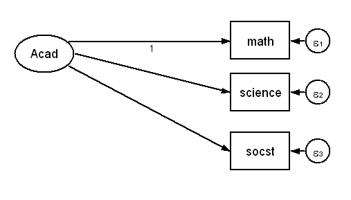
When we looked at the saturated model above we used a very simple model with only observed variables. Now we are going to try to come up with a saturated model that is more closely related to our original model. We will begin by looking at just the measurement part of our model. Here is the diagram.
Followed by the sem code.
sem (Acad->math science socst)

Endogenous variables

Measurement:  math science socst

Exogenous variables

Latent:       Acad

Fitting target model:

Iteration 0:   log likelihood = -2141.1294
Iteration 1:   log likelihood = -2141.1294

Structural equation model                       Number of obs      =       200
Estimation method  = ml
Log likelihood     = -2141.1294

 ( 1)  [math]Acad = 1
------------------------------------------------------------------------------
             |                 OIM
             |      Coef.   Std. Err.      z    P>|z|     [95% Conf. Interval]
-------------+----------------------------------------------------------------
Measurement  |
  math <-    |
        Acad |          1  (constrained)
       _cons |     52.645   .6607911    79.67   0.000     51.34987    53.94013
  -----------+----------------------------------------------------------------
  science <- |
        Acad |   .9027685   .1108342     8.15   0.000     .6855374        1.12
       _cons |      51.85   .6983463    74.25   0.000     50.48127    53.21873
  -----------+----------------------------------------------------------------
  socst <-   |
        Acad |   .8450313    .110572     7.64   0.000     .6283142    1.061748
       _cons |     52.405    .757235    69.21   0.000     50.92085    53.88915
-------------+----------------------------------------------------------------
Variance     |
      e.math |   22.84761   7.002427                      12.53029    41.66011
   e.science |   44.98577   7.024159                      33.12585    61.09185
     e.socst |   68.63626   8.333688                      54.10062    87.07729
        Acad |   64.48137   10.71715                      46.55433    89.31172
------------------------------------------------------------------------------
LR test of model vs. saturated: chi2(0)   =      0.00, Prob > chi2 =      .
As you can see, the measure model with three indicators is itself a saturated model. To be saturated it should have 3*4/2 + 3 = 9 parameters being estimated, which is the case.
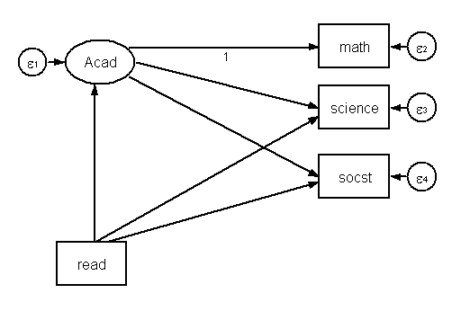
Now, let’s add read to our model like this.
sem (Acad->math science socst)(Acad<-read)(science<-read)(socst<-read), ///
  mean(read) difficult

Endogenous variables

Observed:     science socst
Measurement:  math
Latent:       Acad

Exogenous variables

Observed:     read

Fitting target model:

Iteration 0:   log likelihood =  -3698.205  (not concave)
[output omitted]
Iteration 28:  log likelihood = -2802.3352

Structural equation model                       Number of obs      =       200
Estimation method  = ml
Log likelihood     = -2802.3352

 ( 1)  [math]Acad = 1
-------------------------------------------------------------------------------
              |                 OIM
              |      Coef.   Std. Err.      z    P>|z|     [95% Conf. Interval]
--------------+----------------------------------------------------------------
Structural    |
  science <-  |
         Acad |   .5843354   .3233183     1.81   0.071    -.0493567    1.218028
         read |   .2549117   .2019701     1.26   0.207    -.1409425    .6507659
        _cons |   20.06696   2.821788     7.11   0.000     14.53636    25.59757
  ------------+----------------------------------------------------------------
  socst <-    |
         Acad |   .3945619   .2262457     1.74   0.081    -.0488715    .8379953
         read |   .4119847    .148232     2.78   0.005     .1214554     .702514
        _cons |   18.41618   3.087163     5.97   0.000     12.36546    24.46691
  ------------+----------------------------------------------------------------
  Acad <-     |
         read |   .6051473     .04841    12.50   0.000     .5102655     .700029
--------------+----------------------------------------------------------------
Measurement   |
  math <-     |
         Acad |          1  (constrained)
        _cons |   21.03816    2.57647     8.17   0.000     15.98837    26.08795
--------------+----------------------------------------------------------------
    mean(read)|      52.23   .7231774    72.22   0.000      50.8126     53.6474
--------------+----------------------------------------------------------------
   var(e.math)|   15.32121   18.29777                      1.474762     159.171
var(e.science)|   47.29731   7.818624                      34.20787    65.39535
  var(e.socst)|   65.13928   7.105546                      52.60074    80.66665
   var(e.Acad)|   33.70397   18.81883                      11.28255    100.6827
     var(read)|   104.5971   10.45971                      85.98041    127.2447
-------------------------------------------------------------------------------
LR test of model vs. saturated: chi2(0)   =      0.00, Prob > chi2 =      .
This model has four observed variables. Thus, we should estimate 4*5/2 + 4 = 14 parameters. We achieved this by adding direct paths from read to science and to socst. We could have also achieved the same result by adding two covariances, say e.math*e.science and e.math*e.socst, to our model instead of the direct effects.
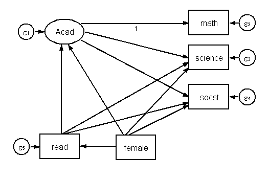
Finally, let’s add female to our model. We now have as many observed variables as our original model.
The above diagram translates to the following code.
sem (Acad -> math science socst)(Acad<-read)(Acad<-female)(read<-female) ///
     (math<- female read)(socst<-female read),                           ///
     mean(female) var(female)

Endogenous variables

Observed:     math socst read
Measurement:  science
Latent:       Acad

Exogenous variables

Observed:     female

Fitting target model:

Iteration 0:   log likelihood = -3111.6647  (not concave)
[output omitted]
Iteration 58:  log likelihood = -2943.2087

Structural equation model                       Number of obs      =       200
Estimation method  = ml
Log likelihood     = -2943.2087

 ( 1)  [math]Acad = 1
------------------------------------------------------------------------------
             |                 OIM
             |      Coef.   Std. Err.      z    P>|z|     [95% Conf. Interval]
-------------+----------------------------------------------------------------
Structural   |
  math <-    |
        read |  -.3219013   .4660796    -0.69   0.490    -1.235401    .5915979
        Acad |          1  (constrained)
      female |   2.990358   2.137855     1.40   0.162    -1.199762    7.180477
       _cons |    20.9637   2.663851     7.87   0.000     15.74265    26.18475
  -----------+----------------------------------------------------------------
  socst <-   |
        read |    .250464   .1525691     1.64   0.101    -.0485661     .549494
        Acad |    .436786   .2230541     1.96   0.050    -.0003919    .8739639
      female |   3.099202    1.37288     2.26   0.024     .4084072    5.789998
       _cons |   17.16439   3.172945     5.41   0.000     10.94553    23.38325
  -----------+----------------------------------------------------------------
  read <-    |
      female |  -1.090232   1.450201    -0.75   0.452    -3.932574     1.75211
       _cons |   52.82418   1.070598    49.34   0.000     50.72584    54.92251
  -----------+----------------------------------------------------------------
  Acad <-    |
        read |   .9273316   .4666623     1.99   0.047     .0126903    1.841973
      female |  -2.880859   2.192737    -1.31   0.189    -7.178543    1.416826
-------------+----------------------------------------------------------------
Measurement  |
  science <- |
        Acad |   .6509763   .3226734     2.02   0.044      .018548    1.283405
       _cons |   21.34222   2.895969     7.37   0.000     15.66623    27.01822
-------------+----------------------------------------------------------------
Mean         |
      female |       .545   .0352119    15.48   0.000      .475986     .614014
-------------+----------------------------------------------------------------
Variance     |
      e.math |   18.69062   14.85898                      3.934787    88.78225
   e.science |   45.08212   7.703921                      32.25118    63.01778
     e.socst |   63.76156   6.970891                      51.46349    78.99847
      e.read |   104.3024   10.43024                      85.73812    126.8862
      e.Acad |   30.33159   15.41889                      11.19933     82.1483
      female |    .247975   .0247975                      .2038392    .3016672
------------------------------------------------------------------------------
LR test of model vs. saturated: chi2(0)   =      0.00, Prob > chi2 =      .
This time there are five observed variables which means that we need to estimate 5*6/2 + 5 = 20 parameters for a saturated model. We did this by adding direct paths from female to Acad, math, and socst and direct paths from read to math and socst. This is the same result that was obtained with the simpler approach used earlier for the saturated model.
The baseline model revisited
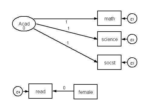
We know that the baseline model estimates five means and five variances and no covariances, because there is only one observed exogenous variables, for a total of 10 total parameters. We can get this from our original model by constraining all of the measurement coefficients (loadings) to be one and all of the path coefficients to be zero. Here is a diagram of the model.
And, here is one way to accomplish this.
sem (Acad ->math@1 science@1 socst@1) (read<-female@0), ///
       var(Acad@0 female) mean(female)

Endogenous variables

Observed:     read
Measurement:  math science socst

Exogenous variables

Observed:     female
Latent:       Acad

Fitting target model:

Iteration 0:   log likelihood = -3257.7854
[omitted output]
Iteration 4:   log likelihood = -3123.7147

Structural equation model                       Number of obs      =       200
Estimation method  = ml
Log likelihood     = -3123.7147

 ( 1)  [math]Acad = 1
 ( 2)  [science]Acad = 1
 ( 3)  [socst]Acad = 1
 ( 4)  [var(Acad)]_cons = 0
------------------------------------------------------------------------------
             |                 OIM
             |      Coef.   Std. Err.      z    P>|z|     [95% Conf. Interval]
-------------+----------------------------------------------------------------
Structural   |
  read <-    |
       _cons |      52.23   .7231774    72.22   0.000      50.8126     53.6474
-------------+----------------------------------------------------------------
Measurement  |
  math <-    |
        Acad |          1  (constrained)
       _cons |     52.645   .6607909    79.67   0.000     51.34987    53.94013
  -----------+----------------------------------------------------------------
  science <- |
        Acad |          1  (constrained)
       _cons |      51.85   .6983462    74.25   0.000     50.48127    53.21873
  -----------+----------------------------------------------------------------
  socst <-   |
        Acad |          1  (constrained)
       _cons |     52.405    .757235    69.21   0.000     50.92085    53.88915
-------------+----------------------------------------------------------------
Mean         |
      female |       .545   .0352119    15.48   0.000      .475986     .614014
-------------+----------------------------------------------------------------
Variance     |
      e.math |   87.32893   8.732889                      71.78572    106.2376
   e.science |   97.53748   9.753746                      80.17729    118.6565
     e.socst |    114.681    11.4681                       94.2695     139.512
      e.read |   104.5971   10.45971                      85.98041    127.2447
      female |    .247975   .0247975                      .2038392    .3016672
        Acad |          0  (constrained)
------------------------------------------------------------------------------
LR test of model vs. saturated: chi2(10)  =    361.01, Prob > chi2 = 0.0000
In this model the term (read<-female@0) estimates an intercept (mean) but no structural coefficient. There is no term that predicting Acad from read which is equivalent to setting that structural coefficient to zero. We added terms for the mean and variance of female. Finally, by convention, the variance of the latent variables is constrained to zero, which we did.

