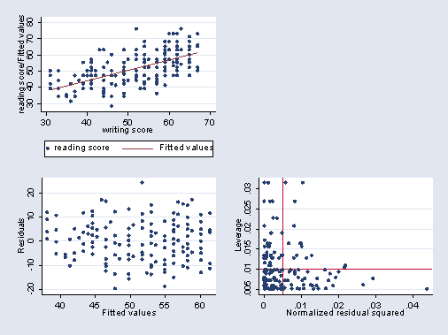
Graphics: Combining Twoway Scatterplots

This module shows examples of combining twoway scatterplots. This is illustrated by showing the command and the resulting graph. This includes hotlinks to the Stata Graphics Manual available over the web and from within Stata by typing help graph.

The data set used in these examples can be obtained using the following command:

use https://stats.idre.ucla.edu/stat/stata/notes/hsb2, clear

This illustrates combining graphs in the following situations.

Plots for separate groups (using by)
Combining separate plots together into a single plot
Combining separate graphs together into a single graph

Plots for separate groups

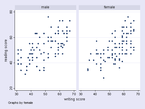
	Separate graphs by gender (male and female) twoway (scatter read write), by(female)

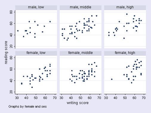
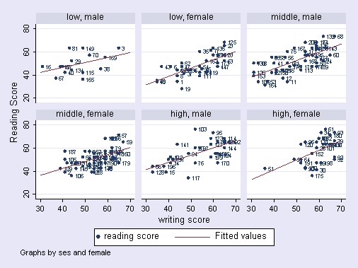
	Separate graphs by ses and gender twoway (scatter read write), by(female ses)

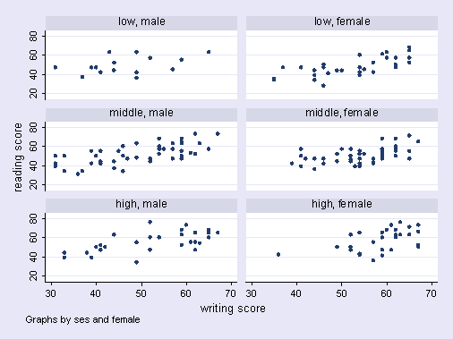
	Swapping position of ses and gender twoway (scatter read write), by(ses female, cols(2))
Combining scatterplots and linear fit in one graph
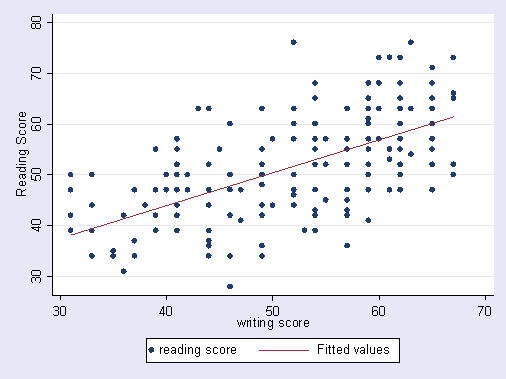
	Scatterplot with linear fit twoway (scatter read write) /// (lfit read write) , /// ytitle(Reading Score)

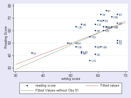
	Graphs separated by SES and female with linear fit lines and points identified by id twoway (scatter read write, mlabel(id)) /// (lfit read write, range(30 70)) , /// ytitle(Reading Score) by(ses female)

	Graph for high ses females with linear fit with and without obs 51 twoway (scatter read write, mlabel(id)) /// (lfit read write, range(30 70)) /// (lfit read write if id != 51, range(30 70)) if female==1 & ses==3,/// ytitle(Reading Score) legend(lab(3 "Fitted values without Obs 51"))
Combining scatterplots with multiple variables and linear fits
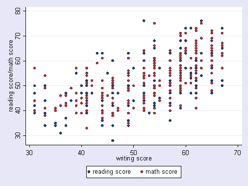
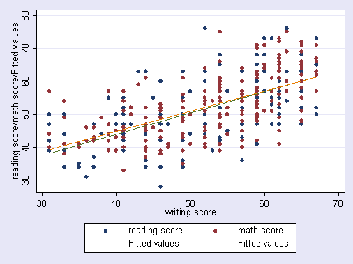
	Reading and math score by writing score twoway (scatter read write) /// (scatter math write)

	Reading and math score by writing score with fit lines twoway (scatter read write) /// (scatter math write) /// (lfit read write) /// (lfit math write)

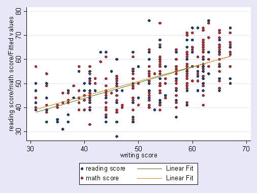
	Adding legend to above graph twoway (scatter read write) /// (scatter math write) /// (lfit read write) /// (lfit math write), /// legend(label(3 "Linear Fit") label(4 "Linear Fit")) /// legend(order(1 3 2 4))

	Final version of graph making line style same as dot style, and ranges the same twoway (scatter read write) /// (scatter math write) /// (lfit read write, pstyle(p1) range(25 80) ) /// (lfit math write, pstyle(p2) range(25 80) ), /// legend(label(3 "Linear Fit") label(4 "Linear Fit")) /// legend(order(1 3 2 4))
Combining scatterplots and linear fit for separate groups
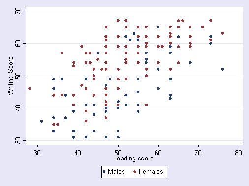
	Overlay graph of males and females in one graph separate write, by(female) twoway (scatter write0 read) (scatter write1 read), /// ytitle(Writing Score) legend(order(1 "Males" 2 "Females"))

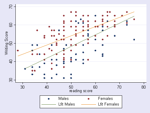
	Overlay graph of males and females in one graph with linear fit lines twoway (scatter write0 read) (scatter write1 read) /// (lfit write0 read) (lfit write1 read), /// ytitle(Writing Score) /// legend(order(1 "Males" 2 "Females" 3 "Lfit Males" 4 "Lfit Females"))
Combining separate graphs into one graph
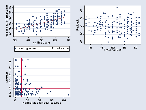
	Making the Graphs First, we make 3 graphs (not shown) twoway (scatter read write) (lfit read write), name(scatter) regress read write rvfplot, name(rvf) lvr2plot, name(lvr) Now we can use graph combine to combine these into one graph, shown below. graph combine scatter rvf lvr

	Combining the graphs differently We can move the place where the empty graph is located, as shown below. graph combine scatter rvf lvr, hole(2)