What to expect from this workshop
Definition of systematic review and meta-analysis
Information on how to collect data for a systematic review and/or meta-analysis
How to organize data for a meta-analysis
How to run a meta-analysis and interpret the results
How to make some useful graphs
A brief discussion of the different types of biases that may compromise the results of a meta-analysis
Resources for further information
All examples will use continuous data; no examples of binary data are presented
What not to expect
This is not an introduction to the use of Stata software
There will be no discussion about how to access and/or use electronic databases
We will not cover any of the more advanced topics, such as meta-regression, multiple imputation of missing data or multilevel meta-analysis
Data file and PowerPoint slides
Example data in Excel Introduction to Meta-analysis in Stata
Introduction
Here’s an experience we can all relate to: you read about a study on your favorite news website, or hear about it on TV or the radio. Some new drug, or treatment, or something, has been shown to do something. Almost always, there is a quote from one of the study’s authors saying something like “this research needs to be replicated with more subjects before anyone should act on the results.” And we all nod our heads, because we know that replication is an important part of the foundation of the scientific method. So let’s say that this topic is something that you really care about, and you wait to hear more results from the replication studies. You find that some of the studies replicated the results while others did not (i.e., failure to replicate results). Now what do you do? You may decide that you are going to find all of the studies on this research question and count up how many found significant results and how many did not. So you do this, but then you notice something that seems a little odd: the greater the number of participants in a study, the more likely the study was to find a statistically significant result. Now to a statistician, this is not surprising at all. In statistics (at least as it is practiced today) “statistical significance” means that the p-value associated with the test statistic is less than .05. And most statisticians realize that this p-value is closely related to the number of participants, which is usually called N. So, in general, as N goes up, the p-value goes down, holding everything else (e.g., alpha, effect size) constant.
But this doesn’t really answer your question. Adding more participants to a study doesn’t make a treatment more or less effective. What you want to know is if the treatment matters in the real world. When you ask a statistician that question, what the statistician hears is “I want to know the effect size.” According to Wikipedia, “in statistics, an effect size is a quantitative measure of the magnitude of a phenomenon” (https://en.wikipedia.org/wiki/Effect_size ). So for example, let’s say that I invented a new drug to lower blood pressure. But if my drug only reduces systolic blood pressure by one point, you say “So what! Your effect size is too small to matter in the real world.” And you would be correct, even if I ran a huge study with thousands of participants to show a statistically significant effect. Later on in this presentation we will cover many different types of effect sizes, but the point here is that you are interested in the size of the effect, not in the statistical significance.
What you did by collecting information from many studies that tried to answer the same research question was a type of meta-analysis. So a meta-analysis is an analysis in which the observations are effect sizes (and estimates of their error) reported in other research, usually published research. Of course, to have “an apples to apples” comparison, you want each of the studies to be addressing a similar, if not the same, research question. You want the outcome measures used to be similar or the same, and the comparison group to be the same. Other things, such as the number of participants, need not be similar across studies.
A systematic review is very similar to a meta-analysis, except the effect sizes (and other values) are not collected from the articles, and hence there is no statistical analysis of these data. Rather, the goal is to give a descriptive summary of the articles. I think of a systematic review as a qualitative version of a meta-analysis.
The dataset that will be used for the examples in this workshop is fictional and contains the means, standard deviations and sample sizes for both an experimental group and a control group. I added in some of the potential complexities that I have seen in meta-analysis datasets that I have used before.
Four related quantities
We need to pause briefly to have a quick discussion about power. There are four related quantities:
- Alpha: the probability of rejecting the null hypothesis when it is true; usually set at 0.05
- Power: the probability of detecting an effect, given that the effect really does exist; either sought (when conducting an a priori power analysis) or observed (after the data have been collected)
- Effect size: quantitative measure of the magnitude of a phenomenon; estimated (when conducting an a priori power analysis) or observed (after the data have been collected)
- N: the number of subjects/participants/observations who participated in a primary research study or are needed for such a study (a power analysis can also be done to determine the number of studies needed in a meta-analysis, but we will be covering that topic in this workshop).
You need to know or estimate three of the four quantities, and the software will calculate the fourth for you. Throughout this workshop, we will be discussing the relationship between these four quantities. Let’s quickly look at a few examples:
- Hold alpha and effect size constant: As N increases, power will increase
- Hold alpha and power constant: As effect size increases, N decreases
- Hold alpha and N constant: As effect size increases, power increases, and so does the probability of finding a statistically-significant effect increases
Guidelines
In many ways, meta-analysis is just like any other type of research. The key to both good research and good meta-analyses is planning. To help with that planning, there are published guidelines on how to conduct good systematic reviews and meta-analyses. It is very important that you review these guidelines before you get started, because you need to collect specific information during the data collection process, and you need to know what that information is. Also, many journals will not publish systematic reviews or meta-analyses if the relevant guidelines were not followed.
Below is a list of the five of the most common guidelines.
- MOOSE: Meta-analysis Of Observational Studies in Epidemiology (http://statswrite.eu/pdf/MOOSE%20Statement.pdf and http://www.ijo.in/documents/14MOOSE_SS.pdf)
- STROBE: Strengthening The Reporting of OBservational studies in Epidemiology (https://www.strobe-statement.org/index.php?id=strobe-home and https://www.strobe-statement.org/index.php?id=available-checklists)
- CONSORT: CONsolidated Standards Of Reporting Trials (http://www.consort-statement.org/ and http://www.equator-network.org/reporting-guidelines/consort/)
- QUOROM: QUality Of Reporting Of Meta-analyses (https://journals.plos.org/plosntds/article/file?type=supplementary&id=info:doi/10.1371/journal.pntd.0000381.s002)
- PRISMA: Preferred Reporting Items for Systematic reviews and Meta-Analyses (http://www.prisma-statement.org/)
There are two organizations that do lots of research and publish many meta-analyses. Because these organizations publish many meta-analyses (and meta-analyses of meta-analyses), they help to set the standards for good meta-analyses. These organizations are the Cochrane Collaboration and the Campbell Collaboration. The Cochrane Collaboration is an organization that collects data related to medicine and health care topics. Because of their focus is on high-quality data for international clients, they do a lot of meta-analyses. Not surprisingly, they wrote a whole book of guidelines on how to conduct both systematic reviews and meta-analyses.
The Campbell Collaboration was founded in 1999 and is named after Donald T. Campbell (the same Don Campbell who co-authored Experimental and Quasi-experimental Designs for Research (Campbell and Stanley, 1963) and Quasi-experimentation: Design and Analysis Issues for Field Settings (Cook and Campbell, 1979)). This organization is like the Cochrane Collaboration, only for social issues. Their site has links to the Cochrane Collaboration guidelines, as well as to other sets of guidelines. Another useful website is from the Countway Library of Medicine: https://guides.library.harvard.edu/meta-analysis/guides .
This sounds like a lot of guidelines, but in truth, they are all very similar. Reading through some of them will give you a good idea of what information is needed in your write up. You will want to know this so that you can collect this information as you move through the data collection process.
Quality checklists
Almost all of the meta-analysis guidelines require that all of the studies included in the meta-analysis be rated on a quality checklist. There are hundreds of quality checklists that you can use. Some have been validated; many have not. You may find that you get different results when you use different quality checklists. The purpose of the quality checklist is to identify studies that are potentially not-so-good and ensure that such studies are not having an undo influence on the results of the meta-analysis. For example, if, according to the quality check list being used, one study was found to be of much lower quality than all of the others in the meta-analysis, you might do a sensitivity analysis in which you omit this study from the meta-analysis and then compare those results to those obtained when it is included in the meta-analysis.
Keep in mind that reporting standards have changed over time – witness the evolution of the American Psychological Association (APA) manuals. This can be an issue in meta-analyses that include studies dating back to the 1990s. Back in the 1990s, it was standard practice to report p-values as being above or below 0.05, but not the exact p-value itself. Also, the requirement to report effect sizes (and their standard errors) is relatively new, so older studies typically did not report them. Some quality checklists, such as the Downs and Black (1998, https://www.ncbi.nlm.nih.gov/pmc/articles/PMC1756728/pdf/v052p00377.pdf ), considered these omissions an indication of a lower-quality study.
To give you a sense of what a quality checklist is like, here are a few example items:
1. Is the hypothesis/aim/objective of the study clearly described? yes = 1; no = 0
20. Were the main outcome measures used accurate (valid and reliable)? yes = 1; no = 0; unable to determine = 0
23. Were study subjects randomized to intervention groups? yes = 1; no = 0; unable to determine = 0
Data collection
Once you are familiar with the guidelines, you are ready to start the data collection process. The first step is to clearly state the research question. This is critical, because it will inform the criterion for what studies will be included in your meta-analysis and which will be excluded. For example, suppose the lead author on the paper is an expert in issues surrounding the gathering of information from children in foster care who had experienced traumatic events. These young people were interviewed as part of legal proceeding related to the traumatic event. Interest may regard the effects of interviewer support on children’s memory and suggestibility. The research question might be: Does interviewer supportiveness improve interview outcomes? This is a very specific question, but oftentimes researchers start with a more general question which gets refined one or more times. Refining the research question may be necessary to increase or decrease the number of studies to be included in the meta-analysis.
Grey literature
When deciding where you will search of articles, you will need to consider if you will include any of the so-called “grey literature” in your search. Grey literature includes articles that are either not published or published in journals that are not-so-easy to access (or journals in which the author paid a publication fee). There is often a question as to whether these articles have undergone the peer-review process. Master’s theses and dissertations are often considered part of the grey literature. Other examples of grey literature include government reports, NGO reports, research/reports from businesses, white papers, conference proceedings/papers, statements by professional organizations, etc. There is some debate as to whether such research should be included in a meta-analysis. On one hand, because these articles have not been through the same type of peer review process that articles published in journals have, they may be of substantially lower quality. (If it wasn’t good enough to be published, why is it good enough to be in my meta-analysis?) Also, it is difficult to access this type of literature, as there is no database to search, and so there may be selection bias with respect to those articles that are discovered and included. On the other hand, some argue that omitting such articles may lead to an inflated estimate of the summary effect size, as the effect sizes reported by grey literature articles will likely be smaller than those reported in published articles.
Inclusion and exclusion criteria
Once the research question has been sufficiently refined, you now need to think about how to determine which studies will be included in your meta-analysis. In practice, instead of developing both inclusion and exclusion criterion, you may just develop exclusion criterion. So you will include all of the research articles you find, unless there is a reason to exclude the article. Here are some examples of exclusion criteria:
- Language: Articles not written in English.
- Date of publication: Articles published before 1980 or after 2016.
- Publication source: Article not published in a peer-reviewed journal.
- Type of research: Did not use an experimental design.
Next, you need to decide where you are going to search for the articles. This is a very important step in the process, because your meta-analysis may be criticized if you don’t search in all possible places and therefore fail to find and include studies that really should be included in the meta-analysis. You decisions regarding the inclusion or exclusion of grey literature becomes very important at this stage, because it will impact where you search for articles.
The next step is to start doing the search of the literature. While ideally you would have a complete list of the exclusion criteria before you start the literature search, the reality is that this may be an iterative process, as you find that items need to be added to the exclusion list as you do the searches. This may mean that some searches need to be done more than once. Remember as you do this to keep track of your search terms for each search, and all of the necessary information for writing up the results. Depending on your research question and your search parameters, you may find very few results or tens of thousands of results. Either of these may lead you to revise your exclusion criteria and/or your search terms.
Sensitivity and specificity
This brings us to the discussion of sensitivity versus specificity. In terms of a meta-analysis, sensitivity means that you get all of what you want. In other words, your search results include all of the articles that should be included in your meta-analysis; nothing is missing. Specificity means that you get none of what you don’t want. In other words, you don’t have articles that shouldn’t be included in your meta-analysis. In practice, when doing the search of the literature, most researchers tend to “error” on the side of sensitivity, to ensure that no relevant study was missed. However, this means more work to sort through the possible studies to eliminate those that should not be included.
Collecting data
Once you have a list of all possible articles to include in the meta-analysis, you need to determine what part of the article you will read in order to determine if the article should be included in the meta-analysis. You will likely have hundreds or thousands of possible articles, so reading each one in its entirety isn’t realistic. Rather, you might read just the abstract, or just the methods section, for example.
Sorting through all of the possible studies takes a lot of time and effort. You need to be very organized so that you don’t end up evaluating the same article multiple times. Usually, this job is done by more than one person. In this situation, some articles need to be evaluated by everyone doing the evaluation task, to ensure that everyone would make the same decision regarding that article (i.e., to include it in the study or not). This should be done early on, in case more training is needed. Consistency between evaluators is critical, and inter-rater agreement needs to be reported.
What information to collect
Before you start collecting the actual data for the meta-analysis, decide which statistical software package will be used to analyze the data. Look at the help file for the command that you will be using. For this workshop, we will be using the meta analysis commands that were introduced in Stata 16. Looking at the help file for meta, you can see that there are several different ways that data file could be structured, depending on the type of data that are available. The meta set command can be used if your dataset contains effects sizes their standard errors or effect sizes their confidence intervals. The meta esize command can be used if your dataset contains the means, standard deviations and sample sizes for two groups (usually an experimental group and a control group). The meta esize command can also be used if your dataset contains the Ns for successes and failures for two groups (for a total of four sample sizes).
With the meta set command, you dataset could be formatted in one of two ways:
esvar sevar
or
es cilvar ciuvar
where “esvar” means “effect size”, “sevar” means “standard error of effect size”, “cilvar” means “confidence interval lower”, and “ciuvar” means “confidence interval upper”.
With the meta esize command, your dataset could be formatted in one of two ways:
Continuous data: n1 mean1 sd1 n2 mean2 sd2
or
Binary outcome with two groups: n11 n12 n21 n22
where “n1” means the sample size for the experimental group, “mean1” means the mean for the experimental group, “sd1” means the standard deviation for the experimental group, “n2” means the sample size for the control group, “mean2” means the mean for the control group, “sd2” means the standard deviation for the control group, “n11” means the number of successes for the experimental group, “n12” means the number of failures for the experimental group, “n21” means the number of successes for the control group, and “n22” means the number of failures for the control group.
As you can see, there are several different ways you can enter data. You want to know which of these you will be using before you start collecting data. For example, in the social sciences, you are likely to find Ns, means and standard deviations in the articles to be included in the meta-analysis. In medical fields, you may be more likely to find odds ratios. Either way, you need to know what information is needed by the software so that you know what to collect. That said, data collection is rarely that straight forward. Because of that, I find that you often end up with two datasets. The first one is the one into which you collect the information that you can find, and the second one is the “cleaned up” one that you use for the analysis. I will describe both of these in more detail a little later on.
Another thing you need to do before starting to collect the data is to determine how you are going to mark the data that you have found. For example, are you going to print out all of the articles and use a highlighter to highlight the needed values? Are you going to have a file of PDFs of the articles and use an electronic highlighter? As mentioned before, if more than one person is going to do this task, you will need to get the inter-rater reliability established before data collection begins.
Another point to consider is the possibility of running a meta-regression. We will not discuss the topic of meta-regressions in this workshop, but the point now is to think about possible covariates that might be included in such a model. You want to think about that before reading through the selected sections of the articles, because you want to collect all of the needed data in as few readings as possible.
Your first dataset may look rather messy and may not be in a form that is ready to be imported into Stata for analysis. This is OK; it is still a good start.
There are still two major issues that need to be addressed: one is the missing data, and the other is the fact that you may have different types of effect sizes from the different studies.
Missing data
As with complex survey data, there are two types of missing data in meta-analyses. The first type is missing studies (akin to unit non-response in survey data). The second type is missing values from a particular study (akin to item non-response). We will deal with missing studies later on when we discuss various types of bias. Here we are going to talk about missing values from the articles. To be clear, how missing data are handled in a meta-analysis can very different from how missing data are handled in almost any other type of research. The “cost” of missing data in a meta-analysis is often high, because there is no way to get more data (because you have already included all of the relevant studies in your meta-analysis), and the number of studies may be rather low.
Before trying to use a more “traditional” form of imputation, such as multiple imputation, in a meta-analysis you can try to find an acceptable method to replace the missing value using the information that is available. One of the best places I have found for information on making these substitutions is the manual for the ES program written by the late Will Shadish. This document describes the formulas used to calculate the different types of effect sizes and describes the consequences of substituting known information for unknown information.
Let’s say that you are collecting Ns, means and standard deviations for your meta-analysis. You must find the N, mean and standard deviation for both the experimental and control group, for a total of six values. One of the articles gives only five values; the N for one of the groups is missing. Now you may be able to figure out what the N is by subtracting the N in one group from the known total sample size, but if you can’t do that, you could just assume that each group had the same N. It turns out the effect size that is calculated with this substitution is very similar what would have been calculated if the real N had been know. Likewise, if you had all but the standard deviation for one group, you might assume that the standard deviations in the two groups were equal. This is a little more of a compromise than assuming equal Ns, but it isn’t too bad. However, you should be hesitant to assume that the means of the two groups were the same.
Let’s say that in another article, the only information that you can find is the value of the F-statistic, the degrees of freedom, and the p-value. You can calculate an effect size from this information. If you can find only the p-value, you can still estimate the effect size. For example, if you have a p-value and the degrees of freedom, you can figure out the t-value, and then calculate an effect size from there. To do this, however, you need to have the exact p-value.
Another method of handling missing data is to contact the author(s) of the study with the missing data and ask for the value or values needed. In my experience, some authors were very understanding and provided the requested values, while others simply ignore such requests. One replied to our email request and said that she would be willing to provide the missing value (which was a mean), but the data were stored on a tape that was no longer readable. There is also the possibility of doing a multiple imputation or possibly a Bayesian meta-analysis, but we will not discuss those topics in this workshop.
Let’s think about missing studies. One of the major concerns with a meta-analysis is collecting all of the relevant research articles, because as we know, not all research is published. Of particular concern are the results of high-quality research that found non-significant results. Finding such research results can be difficult, as such research is published much less often than research that found statistically significant results. So what are your options? You can try to contact researchers who have published articles in this particular area of research to ask about non-published papers. You can search for dissertations or Master’s theses. You can talk to people at academic conferences. You can post inquiries on relevant mailing lists. However, caution must be exercised, because some of these works may be of substantially poorer quality than the work that is published. There could be flaws in the design, instrument construction, data collection techniques, etc. In other words, finding non-significant results isn’t the only reason research is not published.
Once the missing data have been handled and all of the effect sizes have been converted into the same metric, we have our second dataset, which is ready for preliminary analysis.
Different types of effect sizes
There are many different types of effect sizes, some for continuous outcome variables and others for binary outcome variables. The effect sizes for continuous outcome variables belong to one of two families of effect sizes: the d class and the r class. The d class effect sizes are usually calculated from the mean and standard deviation. They are a scaled difference between the means of two group. Glass’ delta, Cohen’s d and Hedges’ g are examples of this type of effect size. Glass’ delta is the difference between the mean of the experimental and control groups divided by the standard deviation of the control group. Cohen’s d is the different between the mean of the experimental and control group divided by the pooled standard deviation (i.e., pooled across the experimental and control groups). Hedges’ g is a correction to Cohen’s d because Cohen’s d tends to overestimate the effect size in small samples (< 10-15 total).
The r class effect sizes are also a ratio, but they are the ratio of variance attributable to an effect divided by the total effect, or more simply, the proportion of variance explained. Examples of this type of effect size include eta-squared and omega-squared.
When dealing with binary data, it is common to have a 2×2 table: event/non-event and treated/controlled.
event non-event
treated A B
control C D
From such a table, three different types of effect sizes can be calculated. These include the risk ratio, the odds ratio and the risk difference.
Risk ratio = (A/n1)/(C/n2)
Odds ratio = (AD)/(BC)
Risk difference = (A/n1) – (C/n2)
The risk ratio and the odds ratio are relative measures, and as such they are relatively insensitive to the number of baseline events. The risk difference is an absolute measure, so it is very sensitive the number of baseline events.
Converting between different types of effect sizes
While you will need to collect information necessary to calculate an effect size from some articles, other articles will provide the effect size. However, there are dozens of different types of effect sizes, so you may need to convert the effect size given in the paper into the type of effect size that you need for your meta-analysis. There are several good online effect size calculators/converters. One of my favorites is: https://www.psychometrica.de/effect_size.html .
You need to be careful when using effect size converters, because some conversions make more sense than others. For example, you can easily convert a Cohen’s d to an odds ratio, but the reverse is not recommended. Why is that? A Cohen’s d is based on data from continuous variables, while an odds ratio is based on data from dichotomous variables. It is easy to make a continuous variable dichotomous, but you can’t make a dichotomous variable continuous (because the dichotomous variable contains less information than the continuous variable). However, Cox (1970) suggested that d(Cox) = LOR/1.65, (where LOR = log odds ratio) and Sanchez-Meca, et. al. (2003) showed that this approximation works well. Bonnet (2007) and Kraemer (2004) have good summaries of issues regarding fourfold tables. Another point to keep in mind is the effect of rounding error when converting between different types of effect sizes.
Like any other quantity calculated from sampled data, an effect size is an estimate. Because it is an estimate, we want to calculate the standard error (or confidence interval) around that estimate. If you give the statistical software the information necessary to calculate the effect size, it will also calculate the standard error for that estimate. However, if you supply the estimate of the effect size, you will also need to supply either the standard error for the estimate or the confidence interval. This can be a real problem when an article reports an effect size but not its standard error, because it may be difficult to find a way to derive that information from what is given in the article.
Despite the large number of effect sizes available, there are still some situations in which there is no agreed-upon measure of effect. Two examples are count models and multilevel models.
Data inspection and descriptive statistics
In the preliminary analysis, we do all of the data checking that you would do with any other dataset, such as looking for errors in the data, getting to know the variables, etc. Of particular interest is looking at the estimates of the effect sizes for outliers. Of course, what counts as an outlier depends on the context, but you still want to identify any extreme effect sizes. If the dataset is small, you can simply look through the data, but if the dataset is large, you may need to use a graph or test to identify outliers. You could use the chi-square test for outliers, the Dixon Q test (1953, 1957) for outliers or the Grubbs (1950, 1969, 1972) test for outliers. Some use a method proposed by Viechtbauer and Cheung, 2010, and there are other methods that could be used as well. One of the common problems is that one test identified a given data point as an outlier, but another test didn’t identify any points as outliers, or would identify a different data point. The other common problem is that if one outlier was removed and the test rerun, a different data point would be identified as an outlier. Especially in small datasets, losing any study for any reason is undesirable. In the end, you may not exclude any of the data points (i.e., effect sizes) identified by any of the techniques because there is no compelling reason to do so (e.g., the effect size had not been miscalculated, the effect size didn’t come from a very different type of study or from measures that were very different from those used in other studies included in the analysis), especially if the value for the data point was not too far beyond the cutoff point for calling the value an outlier. Conducting a sensitivity analyses with and without the “outlier” might be a good idea; hopefully the results won’t be too different.
After you have done the descriptive statistics and considered potential outliers, it is finally time to do the analysis! Before running the meta-analysis, we should discuss three important topics that will be shown in the output. The first is weighting, the second is measures of heterogeneity, and the third is type of model.
Weighting
As we know, some of the studies had more subjects than others. In general, the larger the N, the lower the sampling variability and hence the more precise the estimate. Because of this, the studies with larger Ns are given more weight in a meta-analysis than studies with smaller Ns. This is called “inverse variance weighting”, or in Stata speak, “analytic weighting”. These weights are relative weights and should sum to 100. You do not need to calculate these weights yourself; rather, the software will calculate and use them, and they will be shown in the output.
Heterogeneity
Up to this point, we have focused on finding effect sizes and have considered the variability around these effect sizes, measured by the standard error and/or the confidence interval. This variability is actually comprised of two components: the variation in the true effect sizes, which is called heterogeneity, and spurious variability, which is just random error (e.g., sampling error). When conducting a meta-analysis, we want to get a measure of heterogeneity, or the variation in the true effect sizes. There are several measures of this, and we will discuss each in turn. Please note that the following material is adapted from Chapter 16 of Introduction to Meta-Analysis by Borenstein, Hedges, Higgins and Rothstein (2009, 2021). The explanations found there include useful graphs; reading that chapter is highly recommended.
If the heterogeneity in your meta-analysis dataset was in fact 0, it would mean that all of the studies in the meta-analysis shared the same true effect size. However, we would not expect all of the effect sizes to be the exact same value, because there would still be within-study sampling error. Instead, the effect sizes would fall within a particular range around the true effect.
Now suppose that the true effect size does vary between studies. In this scenario, the observed effect sizes vary for two reasons: Heterogeneity with respect to the true effect sizes and within-study sampling error. Now we need to separate the heterogeneity from the within-study sampling error. The three steps necessary to do this are:
- Compute the total amount of study-to-study variation actually observed
- Estimate how much of the observed effects would be expected to vary from each other if the true effect was actually the same in all studies
- Assume that the excess variation reflects real differences in the effect size (AKA heterogeneity)
Q
Let’s start with the Q statistic, which is a ratio of observed variation to the within-study error, or the heterogeneity in the true effect sizes. Q is referred to as a test of homogeneity in Stata.
$$ Q = \sum_{i=1}^k W_i (Y_i -M)^2$$
In the above equation, Wi is the study weight (1/Vi), Yi is the study effect size, M is the summary effect and k is the number of studies. Alternatively, the formula may be written as
$$ Q = \sum_{i=1}^k \left( \frac{Y_i-M}{S_i} \right)^2$$
Note that you can call Q either a weighted sums of squares (WSS) or a standardized difference (rather like Cohen’s d is a standardized difference).
Looking back at the three steps listed above, the first step is to calculate Q. There is a formula for doing this by hand, but most researchers use a computer program to do this. Once you have Q, the next step is to calculate the expected value of Q, assuming that all studies share a common effect size and hence all of the variation is due to sampling error within studies. Because Q is a standardized measure, the expected value depends only on the degrees of freedom, which is df = k – 1, where k is the number of studies. The third and final step is the find the “excess” variation, which is simply Q – df.
A p-value can be associated with Q. Specifically, the null hypothesis is that all studies share a common effect size, and under this null hypothesis, Q will follow a central chi-squared distribution with degrees of freedom equal to k – 1. As you would expect, this test is sensitive to both the magnitude of the effect (i.e., the excess dispersion), and the precision with which the effect is measured (i.e., the number of studies). While a statistically-significant p-value is evidence that the true effects vary, the converse is not true. In other words, you should not interpret a non-significant result to mean that the true effects do not vary. The result could be non-significant because the true effects do not vary, or because there is not enough power to detect the effect, or some other reason. Also, don’t confuse Q with an estimate of the amount of true variance; other methods can be used for that purpose. Finally, be cautious with Q when you have either a small number of studies in your meta-analysis, and/or lots of with-in study variance, which is often caused by studies with small Ns.
There are some limitations to Q. First of all, the metric is not intuitive. Also, Q is a sum, not a mean, which means that it is very sensitive the number of studies included in the meta-analysis. But calculating Q has not been a waste of time, because it is used in the calculation of other measures of heterogeneity that may be more useful. If we take Q, remove the dependence on the number of studies and return it to the original metric, then we have T2, which is an estimate of variance of the true effects. If we take Q, remove the dependence on the number of studies and express the result as a ratio, we will have I2, which estimates the proportion of the observed variance that is heterogeneity (as opposed to random error).
tau-squared and T2
Now let’s talk about tau-squared and T2. Tau-squared is defined as the variance of the true effect sizes. To know this, we would need to have an infinite number of studies in our meta-analysis, and each of those studies would need to have an infinite number of subjects. In other words, we aren’t going to be able to calculate this value. Rather, we can estimate tau-squared by calculating T2. To do this, we start with (Q – df) and divide this quantity by C.
$$T^2 = \frac{Q-df}{C} $$
where
$$ C = \sum W_i – \frac{\sum W_i^2}{W_i} $$
This puts T2 back into the original metric and makes T2 an average of squared deviations. If tau-squared is the actual value of the variance and T2 is the estimate of that actual value, then you can probably guess that tau is the actual standard deviation and T is the estimate of this parameter. T2 answers the question: how much do the true effect sizes vary?
While tau-squared can never be less than 0 (because the actual variance of the true effects cannot be less than 0), T2 can be less than 0 if the observed variance is less than expected based on the within-study variance (i.e., Q < df). When this happens, T2 should be set to 0.
I2
Notice that T2 and T are absolute measures, meaning that they quantify deviation on the same scale as the effect size index. While this is often useful, it is also useful to have a measure of the proportion of observed variance, so that you can ask questions like “What proportion of the observed variance reflects real differences in effect size?” In their 2003 paper, “Measuring Inconsistency in Meta-analysis”, Higgins, et. al., proposed I2. I2 can be thought of as a type of signal-to-noise ratio.
$$ I^2 = \left( \frac{Q-df}{Q} \right) \times 100\%$$
Alternatively,
$$I^2= \left( \frac{Variance_{bet}}{Variance_{total}} \right) \times 100\% = \left( \frac{\tau^2}{\tau^2+V_Y} \right) \times 100\% $$
In words, I2 is the ratio of excess dispersion to total dispersion. I2 is a descriptive statistic and not an estimate of any underlying quantity; it answers the question: What proportion of the observed variability in effect sizes reflects the variance of the true scores? Borenstein, et. al. note that: “I2 reflects the extent of overlap of confidence intervals, which is dependent on the actual location or spread of the true effects. As such it is convenient to view I2 as a measure of inconsistency across the findings of the studies, and not as a measure of the real variation across the underlying true effects.” (page 118 of the first edition).
Let’s give some examples of interpreting I2. An I2 value near 0 means that most of the observed variance is random; it does not mean that the effects are clustered in a narrow range. For example, the observed effects could vary widely because the studies had a lot of sampling error. On the other hand, an I2 value near 100% indicates that most of the observed variability is real; it does not mean that the effects have a wide range. Instead, they could have a very narrow range and be estimated with great precision. The point here is to stress that I2 is a measure of proportion of variability, not a measure of the amount of true variability.
There are several advantages to using I2. One is that the range is from 0 to 100%, which is independent of the scale of the effect sizes. It can be interpreted as a ratio, similar to indices used in regression and psychometrics. Finally, I2 is not directly influenced by the number of studies included in the meta-analysis.
Because I2 is on a relative scale, you should look at it first to decide if there is enough variation to warrant speculation about the source or cause of the variation. In other words, before jumping into a meta-regression or subgroup analysis, you want to look at I2. If it is really low, then there is no point to doing a meta-regression or subgroup analysis.
H2
H2 is another measure of heterogeneity. The H2 statistic is the ratio of the variance of the estimated overall effect size from a random-effects meta-analysis compared to the variance from a fixed-effects meta-analysis (Lin, Chu and Hodges, 2017). When H2 equals 1, there is perfect homogeneity in the meta-analysis data.
Type of model
Stata (as of version 17) offers three types of meta-analysis models. They are common effect, fixed effects, and random effects.
Common effect: A common effect model assumes that there is one true effect size and that each study effect size equals this true effect size (of course, there may be random or sampling error). In practice, this is a very strong assumption which is often violated.
Fixed effects: A fixed-effects meta-analysis assumes that the observed study effect sizes are different and fixed. All of the studies of interest are assumed to be included in the meta-analysis. This is a strong assumption that may be easily violated. In other words, fixed effect models are appropriate if two conditions are satisfied. The first is that all of the studies included in the meta-analysis are identical in all important aspects. Secondly, the purpose of the analysis is to compute the effect size for a given population, not to generalize the results to other populations. The calculations used in the common-effect model and the fixed-effects model are the same, but the assumptions of the two models are different.
Random effects: A random-effects meta-analysis assumes that the observed study effects are different and random. The studies included in the meta-analysis are a (random and representative) sample of the population of studies of interest. For example, you may think that because the research studies were conducted by independent researchers, there is no reason to believe that the studies are functionally equivalent. Given that the studies gathered data from different subjects, used different interventions and/or different measures, it might not make sense to assume that there is a common effect size. Also, given the differences between the studies, you might want to generalize your results to a range of similar (but not identical) situations or scenarios. Because of the assumptions made by a random-effects model, random effects meta-analysis are often recommended and are frequently seen in the meta-analysis literature.
Stata offers different estimation procedures for each of these types of meta-analysis models. We will look at those available for random-effects models a little later. It is important to note that the calculation of the weight is different for each type of model.
Running the meta-analysis and interpreting the results (including the forest plot)
Let’s return to our example. The cleaned example data in Excel looks like this:
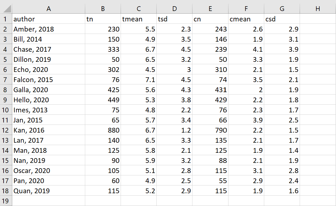
Let’s read the data into Stata using the import excel command. Then we will use the meta esize command to declare the data meta-analysis data. We can also use a few helpful options. The esize(hedgesg) option is used to have the effect sizes calculated as Hedges’ g, which is helpful if some of the study sample sizes are small. The random option is used, and we will discuss this option, and alternatives to this option, shortly. The studylabel option is used so that when the meta-analysis is run, the information in the variable author is included in the output.
clear
import excel "D:\data\Seminars\Stata Meta-analysis\example_data.xlsx", sheet("Sheet1") firstrow

meta esize tn tmean tsd cn cmean csd, esize(hedgesg) random studylabel(author)

Meta-analysis setting information

Study information
No. of studies: 17
Study label: author
Study size: _meta_studysize
Summary data: tn tmean tsd cn cmean csd

Effect size
Type: hedgesg
Label: Hedges's g
Variable: _meta_es
Bias correction: Approximate

Precision
Std. err.: _meta_se
Std. err. adj.: None
CI: [_meta_cil, _meta_ciu]
CI level: 95%

Model and method
Model: Random effects
Method: REML
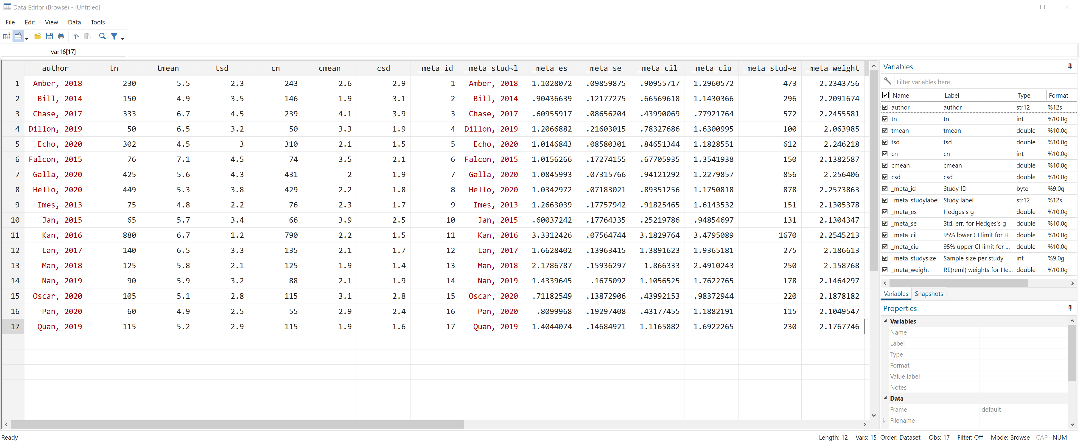
The meta esize command caused Stata to create several new variables in the dataset. All of the new variables start with an underscore (_). Let’s use the browse command to have a look.
We will use the meta summarize command to run the meta-analysis. Notice that Stata uses the variables that it created to run the meta-analysis.
meta summarize, random

  Effect-size label: Hedges's g
        Effect size: _meta_es
          Std. err.: _meta_se
        Study label: author

Meta-analysis summary                     Number of studies =     17
Random-effects model                      Heterogeneity:
Method: REML                                          tau2 =  0.4378
                                                    I2 (%) =   97.14
                                                        H2 =   34.96

--------------------------------------------------------------------
            Study |     Hedges's g    [95% conf. interval]  % weight
------------------+-------------------------------------------------
      Amber, 2018 |          1.103       0.910       1.296      6.02
       Bill, 2014 |          0.904       0.666       1.143      5.95
      Chase, 2017 |          0.610       0.440       0.779      6.05
     Dillon, 2019 |          1.207       0.783       1.630      5.56
       Echo, 2020 |          1.015       0.847       1.183      6.05
     Falcon, 2015 |          1.016       0.677       1.354      5.76
      Galla, 2020 |          1.085       0.941       1.228      6.08
      Hello, 2020 |          1.034       0.894       1.175      6.08
       Imes, 2013 |          1.266       0.918       1.614      5.74
        Jan, 2015 |          0.600       0.252       0.949      5.74
        Kan, 2016 |          3.331       3.183       3.480      6.07
        Lan, 2017 |          1.663       1.389       1.937      5.89
        Man, 2018 |          2.179       1.866       2.491      5.81
        Nan, 2019 |          1.434       1.106       1.762      5.78
      Oscar, 2020 |          0.712       0.440       0.984      5.89
        Pan, 2020 |          0.810       0.432       1.188      5.67
       Quan, 2019 |          1.404       1.117       1.692      5.86
------------------+-------------------------------------------------
            theta |          1.260       0.938       1.582
--------------------------------------------------------------------
Test of theta = 0: z = 7.68                      Prob > |z| = 0.0000
Test of homogeneity: Q = chi2(16) = 910.19         Prob > Q = 0.0000
Let’s go through each part of the output. At the top, we see the header information. This reminds us that Hedges’ g is the type of effect size, that the variable in the dataset that contains the effect sizes is _meta_es, that the variable in the dataset that contains the standard error of the effect size is _meta_se, and that the variable in the dataset that contains the study label is the variable author. On the left, we can see that a random-effects model was run using the method REML (restricted maximum likelihood), which is the default estimation method for meta-analysis in Stata. On the right, we can see that 17 studies were included in the analysis, and we have three measures of heterogeneity: tau-squared, I2 and H2. In the table, we see one line for each study included in the analysis. The information that is in the left-most column is the information that is contained in the variable specified in studylabel option on the meta esize command. I usually include the date of the study because I like that information to be shown in this type of table and in the forest plot (which we will get to soon). The effect size is given in the next column, and then the lower and upper 95% confidence interval. In the column on the right is the weight. Although not shown in the output, the weights sum to 100. At the bottom of the table, we see that theta equals 1.260, with a 95% confidence interval of 0.938 to 1.582. Under the table, we have the test of theta = 0 (z = 7.68) and the corresponding p-value (0.0000). Under that, we see the test of Q (chi-square test) and its p-value. In this example, the chi-square test on 16 degrees of freedom equals 910.19, and the corresponding p-value is 0.0000. These results indicate that the overall effect size, 1.260, is different from 0, and that there is heterogeneity in the data.
The table above is nice, but let’s see the forest plot, which is another common way to present the results of a meta-analysis. We will use the meta forestplot command.
meta forestplot
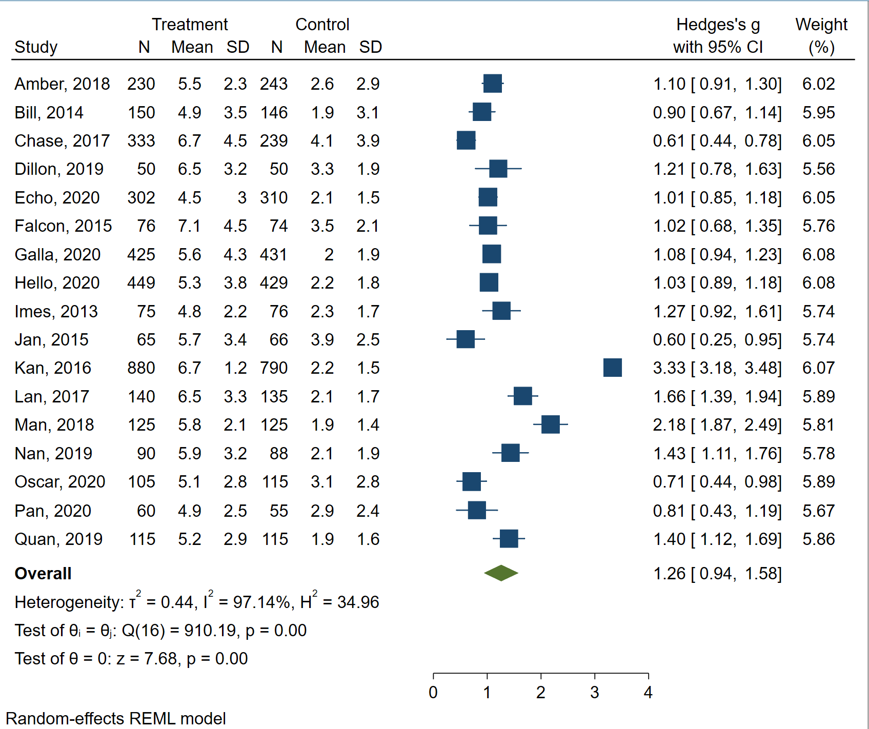
The forest plot contains all of the information that was given in the table above, plus some. Now we can see the data, a plot of the data with lines indicating the 95% confidence intervals, and more measures of heterogeneity. Of course, this graph can be customized for publication, if necessary.
Looking at the graph (or the table above), one may wonder if the results are unduly influenced by the Kan, 2016 study. A Galbraith plot may be helpful here.
meta galbraithplot
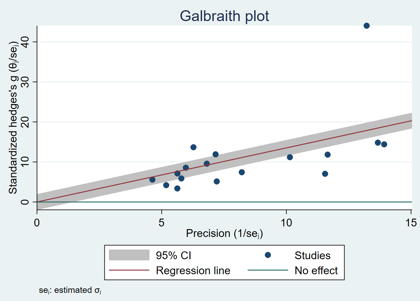
It is clear from the plot above that there is an outlier. The Kan, 2016 study has the largest sample size of any study (880), and it has the largest estimated effect size (3.33). Let’s try a sensitivity analysis to see if the results change when this study is omitted from the analysis.
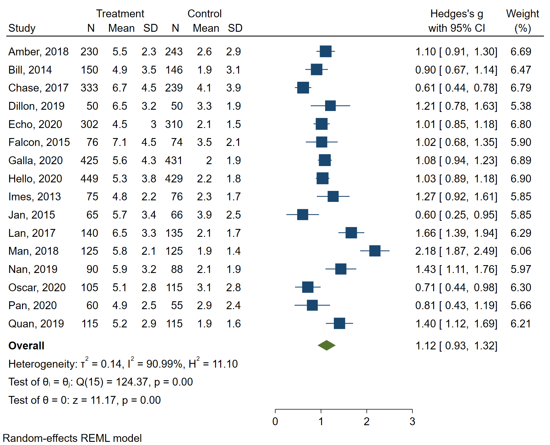
When the Kan, 2016 study is omitted, the estimated overall effect size drops from 1.26 to 1.12. Both values are different from 0. Each of the measures of heterogeneity decrease, although I2 does not decrease by much. Given these results, it seems that the Kan, 2016 study does not unduly influence the results.
Stata offers another way to look at this. We can use the leaveoneout option on either the meta summarize or the meta forestplot command. The leaveoneout option runs the meta-analysis as many times as there are studies in the analysis, each time leaving out each study in turn. This is one way to search for outliers.
meta forestplot, leaveoneout

All of the effect sizes and confidence intervals look pretty similar, indicating that no study appears to be an outlier.
Although the assumptions of common-effect and fixed-effects models may be strong and often violated in practice, let’s run each type of model with our example data to see how the results differ. We will show the table from each analysis.
meta summarize, common

  Effect-size label: Hedges's g
        Effect size: _meta_es
          Std. err.: _meta_se
        Study label: author

Meta-analysis summary                     Number of studies =     17
Common-effect model
Method: Inverse-variance

--------------------------------------------------------------------
            Study |     Hedges's g    [95% conf. interval]  % weight
------------------+-------------------------------------------------
      Amber, 2018 |          1.103       0.910       1.296      7.54
       Bill, 2014 |          0.904       0.666       1.143      4.94
      Chase, 2017 |          0.610       0.440       0.779      9.78
     Dillon, 2019 |          1.207       0.783       1.630      1.57
       Echo, 2020 |          1.015       0.847       1.183      9.95
     Falcon, 2015 |          1.016       0.677       1.354      2.46
      Galla, 2020 |          1.085       0.941       1.228     13.69
      Hello, 2020 |          1.034       0.894       1.175     14.20
       Imes, 2013 |          1.266       0.918       1.614      2.32
        Jan, 2015 |          0.600       0.252       0.949      2.32
        Kan, 2016 |          3.331       3.183       3.480     12.80
        Lan, 2017 |          1.663       1.389       1.937      3.76
        Man, 2018 |          2.179       1.866       2.491      2.89
        Nan, 2019 |          1.434       1.106       1.762      2.61
      Oscar, 2020 |          0.712       0.440       0.984      3.81
        Pan, 2020 |          0.810       0.432       1.188      1.97
       Quan, 2019 |          1.404       1.117       1.692      3.40
------------------+-------------------------------------------------
            theta |          1.351       1.298       1.404
--------------------------------------------------------------------
Test of theta = 0: z = 49.91                     Prob > |z| = 0.0000

meta summarize, fixed

  Effect-size label: Hedges's g
        Effect size: _meta_es
          Std. err.: _meta_se
        Study label: author

Meta-analysis summary                     Number of studies =     17
Fixed-effects model                       Heterogeneity:
Method: Inverse-variance                            I2 (%) =   98.24
                                                        H2 =   56.89

--------------------------------------------------------------------
            Study |     Hedges's g    [95% conf. interval]  % weight
------------------+-------------------------------------------------
      Amber, 2018 |          1.103       0.910       1.296      7.54
       Bill, 2014 |          0.904       0.666       1.143      4.94
      Chase, 2017 |          0.610       0.440       0.779      9.78
     Dillon, 2019 |          1.207       0.783       1.630      1.57
       Echo, 2020 |          1.015       0.847       1.183      9.95
     Falcon, 2015 |          1.016       0.677       1.354      2.46
      Galla, 2020 |          1.085       0.941       1.228     13.69
      Hello, 2020 |          1.034       0.894       1.175     14.20
       Imes, 2013 |          1.266       0.918       1.614      2.32
        Jan, 2015 |          0.600       0.252       0.949      2.32
        Kan, 2016 |          3.331       3.183       3.480     12.80
        Lan, 2017 |          1.663       1.389       1.937      3.76
        Man, 2018 |          2.179       1.866       2.491      2.89
        Nan, 2019 |          1.434       1.106       1.762      2.61
      Oscar, 2020 |          0.712       0.440       0.984      3.81
        Pan, 2020 |          0.810       0.432       1.188      1.97
       Quan, 2019 |          1.404       1.117       1.692      3.40
------------------+-------------------------------------------------
            theta |          1.351       1.298       1.404
--------------------------------------------------------------------
Test of theta = 0: z = 49.91                     Prob > |z| = 0.0000
Test of homogeneity: Q = chi2(16) = 910.19         Prob > Q = 0.0000

meta summarize, random

  Effect-size label: Hedges's g
        Effect size: _meta_es
          Std. err.: _meta_se
        Study label: author

Meta-analysis summary                     Number of studies =     17
Random-effects model                      Heterogeneity:
Method: REML                                          tau2 =  0.4378
                                                    I2 (%) =   97.14
                                                        H2 =   34.96

--------------------------------------------------------------------
            Study |     Hedges's g    [95% conf. interval]  % weight
------------------+-------------------------------------------------
      Amber, 2018 |          1.103       0.910       1.296      6.02
       Bill, 2014 |          0.904       0.666       1.143      5.95
      Chase, 2017 |          0.610       0.440       0.779      6.05
     Dillon, 2019 |          1.207       0.783       1.630      5.56
       Echo, 2020 |          1.015       0.847       1.183      6.05
     Falcon, 2015 |          1.016       0.677       1.354      5.76
      Galla, 2020 |          1.085       0.941       1.228      6.08
      Hello, 2020 |          1.034       0.894       1.175      6.08
       Imes, 2013 |          1.266       0.918       1.614      5.74
        Jan, 2015 |          0.600       0.252       0.949      5.74
        Kan, 2016 |          3.331       3.183       3.480      6.07
        Lan, 2017 |          1.663       1.389       1.937      5.89
        Man, 2018 |          2.179       1.866       2.491      5.81
        Nan, 2019 |          1.434       1.106       1.762      5.78
      Oscar, 2020 |          0.712       0.440       0.984      5.89
        Pan, 2020 |          0.810       0.432       1.188      5.67
       Quan, 2019 |          1.404       1.117       1.692      5.86
------------------+-------------------------------------------------
            theta |          1.260       0.938       1.582
--------------------------------------------------------------------
Test of theta = 0: z = 7.68                      Prob > |z| = 0.0000
Test of homogeneity: Q = chi2(16) = 910.19         Prob > Q = 0.0000
The effect sizes and confidence intervals are the same across all three models, but the weights and the measures of heterogeneity are different. In the common-effect model, there are no measures of heterogeneity, and in the fixed-effects model, there is no measure of tau-squared. The value of I2 is similar in the fixed-effects and random-effects models, but the value of H2 is quite different. The value of theta is the same in the common-effect and fixed-effects models (1.351) but different in the random-effects model (1.260). The purpose of this demonstration is to show that the three types of models yield different results. You should choose between these types of models based on the assumptions that you believe to be true about your data, rather than the results given.
Now let’s look at the different estimation methods that are available for random-effects models. Stata currently offers six. The following definitions are quoted directly from the Stata 17 meta-analysis documentation, page 7. The nometashow option is used to suppress the display of the variables used in the meta-analysis.
REML, ML, and EB assume that the distribution of random effects is normal. The other estimators make no distributional assumptions about random effects.
The REML method (Raudenbush 2009) produces an unbiased, nonnegative estimate of tau-squared and is commonly used in practice. (It is the default estimation method in Stata because it performs well in most scenarios.)
meta summarize, random(reml) nometashow

Meta-analysis summary                     Number of studies =     17
Random-effects model                      Heterogeneity:
Method: REML                                          tau2 =  0.4378
                                                    I2 (%) =   97.14
                                                        H2 =   34.96

--------------------------------------------------------------------
            Study |     Hedges's g    [95% conf. interval]  % weight
------------------+-------------------------------------------------
      Amber, 2018 |          1.103       0.910       1.296      6.02
       Bill, 2014 |          0.904       0.666       1.143      5.95
      Chase, 2017 |          0.610       0.440       0.779      6.05
     Dillon, 2019 |          1.207       0.783       1.630      5.56
       Echo, 2020 |          1.015       0.847       1.183      6.05
     Falcon, 2015 |          1.016       0.677       1.354      5.76
      Galla, 2020 |          1.085       0.941       1.228      6.08
      Hello, 2020 |          1.034       0.894       1.175      6.08
       Imes, 2013 |          1.266       0.918       1.614      5.74
        Jan, 2015 |          0.600       0.252       0.949      5.74
        Kan, 2016 |          3.331       3.183       3.480      6.07
        Lan, 2017 |          1.663       1.389       1.937      5.89
        Man, 2018 |          2.179       1.866       2.491      5.81
        Nan, 2019 |          1.434       1.106       1.762      5.78
      Oscar, 2020 |          0.712       0.440       0.984      5.89
        Pan, 2020 |          0.810       0.432       1.188      5.67
       Quan, 2019 |          1.404       1.117       1.692      5.86
------------------+-------------------------------------------------
            theta |          1.260       0.938       1.582
--------------------------------------------------------------------
Test of theta = 0: z = 7.68                      Prob > |z| = 0.0000
Test of homogeneity: Q = chi2(16) = 910.19         Prob > Q = 0.0000
When the number of studies is large, the ML method (Hardy and Thompson 1998; Thompson and Sharp 1999) is more efficient than the REML method but may produce biased estimates when the number of studies is small, which is a common case in meta-analysis.
meta summarize, random(mle) nometashow

Meta-analysis summary                     Number of studies =     17
Random-effects model                      Heterogeneity:
Method: ML                                            tau2 =  0.4118
                                                    I2 (%) =   96.96
                                                        H2 =   32.94

--------------------------------------------------------------------
            Study |     Hedges's g    [95% conf. interval]  % weight
------------------+-------------------------------------------------
      Amber, 2018 |          1.103       0.910       1.296      6.03
       Bill, 2014 |          0.904       0.666       1.143      5.95
      Chase, 2017 |          0.610       0.440       0.779      6.06
     Dillon, 2019 |          1.207       0.783       1.630      5.54
       Echo, 2020 |          1.015       0.847       1.183      6.06
     Falcon, 2015 |          1.016       0.677       1.354      5.75
      Galla, 2020 |          1.085       0.941       1.228      6.09
      Hello, 2020 |          1.034       0.894       1.175      6.09
       Imes, 2013 |          1.266       0.918       1.614      5.73
        Jan, 2015 |          0.600       0.252       0.949      5.73
        Kan, 2016 |          3.331       3.183       3.480      6.08
        Lan, 2017 |          1.663       1.389       1.937      5.89
        Man, 2018 |          2.179       1.866       2.491      5.81
        Nan, 2019 |          1.434       1.106       1.762      5.77
      Oscar, 2020 |          0.712       0.440       0.984      5.89
        Pan, 2020 |          0.810       0.432       1.188      5.66
       Quan, 2019 |          1.404       1.117       1.692      5.86
------------------+-------------------------------------------------
            theta |          1.260       0.948       1.572
--------------------------------------------------------------------
Test of theta = 0: z = 7.91                      Prob > |z| = 0.0000
Test of homogeneity: Q = chi2(16) = 910.19         Prob > Q = 0.0000
The EB estimator (Berkey et al. 1995), also known as the Paule–Mandel estimator (Paule and Mandel 1982), tends to be less biased than other RE methods, but it is also less efficient than REML or DL (Knapp and Hartung 2003).
meta summarize, random(ebayes) nometashow

Meta-analysis summary                     Number of studies =     17
Random-effects model                      Heterogeneity:
Method: Empirical Bayes                               tau2 =  0.4296
                                                    I2 (%) =   97.09
                                                        H2 =   34.32

--------------------------------------------------------------------
            Study |     Hedges's g    [95% conf. interval]  % weight
------------------+-------------------------------------------------
      Amber, 2018 |          1.103       0.910       1.296      6.02
       Bill, 2014 |          0.904       0.666       1.143      5.95
      Chase, 2017 |          0.610       0.440       0.779      6.05
     Dillon, 2019 |          1.207       0.783       1.630      5.55
       Echo, 2020 |          1.015       0.847       1.183      6.05
     Falcon, 2015 |          1.016       0.677       1.354      5.76
      Galla, 2020 |          1.085       0.941       1.228      6.08
      Hello, 2020 |          1.034       0.894       1.175      6.08
       Imes, 2013 |          1.266       0.918       1.614      5.74
        Jan, 2015 |          0.600       0.252       0.949      5.74
        Kan, 2016 |          3.331       3.183       3.480      6.08
        Lan, 2017 |          1.663       1.389       1.937      5.89
        Man, 2018 |          2.179       1.866       2.491      5.81
        Nan, 2019 |          1.434       1.106       1.762      5.78
      Oscar, 2020 |          0.712       0.440       0.984      5.89
        Pan, 2020 |          0.810       0.432       1.188      5.67
       Quan, 2019 |          1.404       1.117       1.692      5.86
------------------+-------------------------------------------------
            theta |          1.260       0.941       1.579
--------------------------------------------------------------------
Test of theta = 0: z = 7.75                      Prob > |z| = 0.0000
Test of homogeneity: Q = chi2(16) = 910.19         Prob > Q = 0.0000
The DL method (DerSimonian and Laird 1986), historically, is one of the most popular estimation methods because it does not make any assumptions about the distribution of the random effects and does not require iteration. But it may underestimate tau-squared, especially when the variability is large and the number of studies is small. However, when the variability is not too large and the studies are of similar sizes, this estimator is more efficient than other noniterative estimators HE and SJ.
meta summarize, random(dlaird) nometashow

Meta-analysis summary                     Number of studies =     17
Random-effects model                      Heterogeneity:
Method: DerSimonian–Laird                             tau2 =  0.7206
                                                    I2 (%) =   98.24
                                                        H2 =   56.89

--------------------------------------------------------------------
            Study |     Hedges's g    [95% conf. interval]  % weight
------------------+-------------------------------------------------
      Amber, 2018 |          1.103       0.910       1.296      5.97
       Bill, 2014 |          0.904       0.666       1.143      5.93
      Chase, 2017 |          0.610       0.440       0.779      5.98
     Dillon, 2019 |          1.207       0.783       1.630      5.68
       Echo, 2020 |          1.015       0.847       1.183      5.99
     Falcon, 2015 |          1.016       0.677       1.354      5.81
      Galla, 2020 |          1.085       0.941       1.228      6.00
      Hello, 2020 |          1.034       0.894       1.175      6.00
       Imes, 2013 |          1.266       0.918       1.614      5.79
        Jan, 2015 |          0.600       0.252       0.949      5.79
        Kan, 2016 |          3.331       3.183       3.480      6.00
        Lan, 2017 |          1.663       1.389       1.937      5.89
        Man, 2018 |          2.179       1.866       2.491      5.84
        Nan, 2019 |          1.434       1.106       1.762      5.82
      Oscar, 2020 |          0.712       0.440       0.984      5.89
        Pan, 2020 |          0.810       0.432       1.188      5.75
       Quan, 2019 |          1.404       1.117       1.692      5.87
------------------+-------------------------------------------------
            theta |          1.259       0.850       1.668
--------------------------------------------------------------------
Test of theta = 0: z = 6.03                      Prob > |z| = 0.0000
Test of homogeneity: Q = chi2(16) = 910.19         Prob > Q = 0.0000
The SJ estimator (Sidik and Jonkman 2005), along with the EB estimator, is the best estimator in terms of bias for large tau-squared (Sidik and Jonkman 2007). This method always produces a positive estimate of tau-squared and thus does not need truncating at 0, unlike the other noniterative methods.
meta summarize, random(sjonkman) nometashow

Meta-analysis summary                     Number of studies =     17
Random-effects model                      Heterogeneity:
Method: Sidik–Jonkman                                 tau2 =  0.4292
                                                    I2 (%) =   97.08
                                                        H2 =   34.29

--------------------------------------------------------------------
            Study |     Hedges's g    [95% conf. interval]  % weight
------------------+-------------------------------------------------
      Amber, 2018 |          1.103       0.910       1.296      6.02
       Bill, 2014 |          0.904       0.666       1.143      5.95
      Chase, 2017 |          0.610       0.440       0.779      6.05
     Dillon, 2019 |          1.207       0.783       1.630      5.55
       Echo, 2020 |          1.015       0.847       1.183      6.05
     Falcon, 2015 |          1.016       0.677       1.354      5.76
      Galla, 2020 |          1.085       0.941       1.228      6.08
      Hello, 2020 |          1.034       0.894       1.175      6.08
       Imes, 2013 |          1.266       0.918       1.614      5.74
        Jan, 2015 |          0.600       0.252       0.949      5.74
        Kan, 2016 |          3.331       3.183       3.480      6.08
        Lan, 2017 |          1.663       1.389       1.937      5.89
        Man, 2018 |          2.179       1.866       2.491      5.81
        Nan, 2019 |          1.434       1.106       1.762      5.78
      Oscar, 2020 |          0.712       0.440       0.984      5.89
        Pan, 2020 |          0.810       0.432       1.188      5.67
       Quan, 2019 |          1.404       1.117       1.692      5.86
------------------+-------------------------------------------------
            theta |          1.260       0.941       1.579
--------------------------------------------------------------------
Test of theta = 0: z = 7.75                      Prob > |z| = 0.0000
Test of homogeneity: Q = chi2(16) = 910.19         Prob > Q = 0.0000
Like DL, the HE estimator (Hedges 1983) is a method of moments estimator, but, unlike DL, it does not weight effect-size variance estimates (DerSimonian and Laird 1986). Veroniki et al. (2016) note, however, that this method is not widely used in practice.
meta summarize, random(hedges) nometashow

Meta-analysis summary                     Number of studies =     17
Random-effects model                      Heterogeneity:
Method: Hedges                                        tau2 =  0.4211
                                                    I2 (%) =   97.03
                                                        H2 =   33.66

--------------------------------------------------------------------
            Study |     Hedges's g    [95% conf. interval]  % weight
------------------+-------------------------------------------------
      Amber, 2018 |          1.103       0.910       1.296      6.02
       Bill, 2014 |          0.904       0.666       1.143      5.95
      Chase, 2017 |          0.610       0.440       0.779      6.05
     Dillon, 2019 |          1.207       0.783       1.630      5.55
       Echo, 2020 |          1.015       0.847       1.183      6.06
     Falcon, 2015 |          1.016       0.677       1.354      5.75
      Galla, 2020 |          1.085       0.941       1.228      6.08
      Hello, 2020 |          1.034       0.894       1.175      6.09
       Imes, 2013 |          1.266       0.918       1.614      5.73
        Jan, 2015 |          0.600       0.252       0.949      5.73
        Kan, 2016 |          3.331       3.183       3.480      6.08
        Lan, 2017 |          1.663       1.389       1.937      5.89
        Man, 2018 |          2.179       1.866       2.491      5.81
        Nan, 2019 |          1.434       1.106       1.762      5.78
      Oscar, 2020 |          0.712       0.440       0.984      5.89
        Pan, 2020 |          0.810       0.432       1.188      5.66
       Quan, 2019 |          1.404       1.117       1.692      5.86
------------------+-------------------------------------------------
            theta |          1.260       0.944       1.576
--------------------------------------------------------------------
Test of theta = 0: z = 7.82                      Prob > |z| = 0.0000
Test of homogeneity: Q = chi2(16) = 910.19         Prob > Q = 0.0000
The HS estimator (Schmidt and Hunter 2015) is negatively biased and thus not recommended when unbiasedness is important (Viechtbauer 2005). Otherwise, the mean squared error of HS is similar to that of ML and is smaller than those of HE, DL, and REML.
meta summarize, random(hschmidt) nometashow

Meta-analysis summary                     Number of studies =     17
Random-effects model                      Heterogeneity:
Method: Hunter–Schmidt                                tau2 =  0.6544
                                                    I2 (%) =   98.07
                                                        H2 =   51.76

--------------------------------------------------------------------
            Study |     Hedges's g    [95% conf. interval]  % weight
------------------+-------------------------------------------------
      Amber, 2018 |          1.103       0.910       1.296      5.97
       Bill, 2014 |          0.904       0.666       1.143      5.93
      Chase, 2017 |          0.610       0.440       0.779      5.99
     Dillon, 2019 |          1.207       0.783       1.630      5.66
       Echo, 2020 |          1.015       0.847       1.183      6.00
     Falcon, 2015 |          1.016       0.677       1.354      5.80
      Galla, 2020 |          1.085       0.941       1.228      6.01
      Hello, 2020 |          1.034       0.894       1.175      6.02
       Imes, 2013 |          1.266       0.918       1.614      5.78
        Jan, 2015 |          0.600       0.252       0.949      5.78
        Kan, 2016 |          3.331       3.183       3.480      6.01
        Lan, 2017 |          1.663       1.389       1.937      5.89
        Man, 2018 |          2.179       1.866       2.491      5.84
        Nan, 2019 |          1.434       1.106       1.762      5.81
      Oscar, 2020 |          0.712       0.440       0.984      5.89
        Pan, 2020 |          0.810       0.432       1.188      5.74
       Quan, 2019 |          1.404       1.117       1.692      5.87
------------------+-------------------------------------------------
            theta |          1.259       0.869       1.649
--------------------------------------------------------------------
Test of theta = 0: z = 6.32                      Prob > |z| = 0.0000
Test of homogeneity: Q = chi2(16) = 910.19         Prob > Q = 0.0000
In this example, all the results are very similar. That will not be true for all meta-analysis datasets, especially smaller datasets. It is important to report the type of model run and the estimator used.
Potential sources of bias
In this section, we will discuss some sources of potential bias.
As mentioned previously, it is really important to include all of the relevant studies in a meta-analysis. However, some may be unobtainable because of some type of bias. One type of bias is publication bias. Publication bias is the bias by publishers of academic journals to prefer to publish studies reporting statistically significant results rather than studies reporting statistically non-significant results. In a similar vein, researchers may be loath to write up a paper reporting statistically non-significant results on the belief that the paper is more likely to be rejected. The effect on a meta-analysis is that there could be missing data (i.e., unit non-response), and these missing data bias the sample of studies included in the meta-analysis. This, of course, leads to a biased estimate of the summary effect. One other point to keep in mind: For any given sample size, the result is more likely to be statistically significant if the effect size is large. Hence, publication bias refers to both statistically significant results and large effect sizes. There are other types of bias that should also be considered. These include:
-
- Language bias: English-language databases and journals are more likely to be searched (does someone on your research team speak/read another language, and do you have access to journals in that language?)
-
- Availability bias: including those studies that are easiest for the meta-analyst to access (To which journals/databases does your university subscribe?)
-
- Cost bias: including those studies that are freely available or lowest cost (To which journals/databases does your university subscribe?)
-
- Familiarity bias: including studies from one’s own field of research (an advantage to having an interdisciplinary research team)
-
- Duplication bias: multiple similar studies reporting statistical significance are more likely to published (checking reference sections for articles)
-
- Citation bias: studies with statistically significant results are more likely to be cited and hence easier to find (checking reference sections for articles)
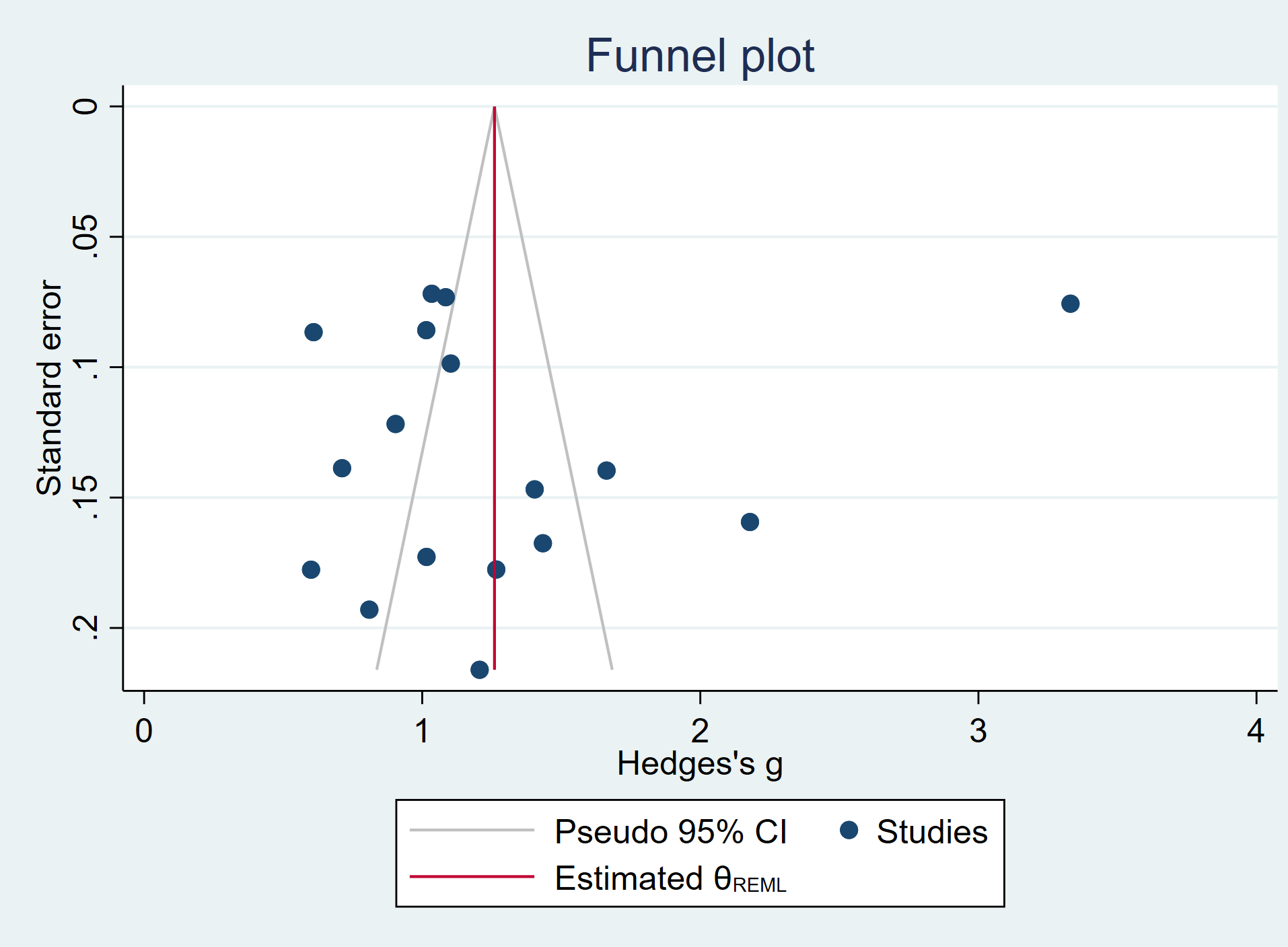
A funnel plot is a good way to start looking for potential bias. Ideally, the dots on the funnel plot, which represent the studies in the meta-analysis, will be (approximately) symmetrical around the mean of the effect size. There is usually a line on the plot indicating this mean. If the dots are not symmetrical, then there may be some sort of bias because studies with certain effect sizes (usually small effect sizes) are missing. This used to be referred to as publication bias, but that term is not used much currently because the omitted studies may be missing for other reasons.
Let’s look at a funnel plot of our example data. The effect size is usually on the x-axis and the sample size or variance on the y-axis with the largest sample size or smallest variance at the top. If there is no bias, then the studies will be distributed evenly around the mean effect size. Smaller studies will appear near the bottom because they will have more variance than the larger studies (which are at the top of the graph). If there is bias, then there will seem to be studies missing from the middle left of the graph, and very few, if any, studies in the lower left of the graph. (The lower left being where small studies reporting small effect sizes would be.)
In the plot below, there may be some missing studies (notice the “hole” to the right of the red line between standard error values of about 0.16 to 0.06).
meta funnelplot, random
A contour funnel plot can also be made using the contour option. The numbers in parentheses give the range of p-values.
meta funnelplot, random contours(1 5 10)
problem with graph
Small-study effects
Sterne, et. al. (2001) coined the term “small study effect” to describe the phenomenon that smaller (published) studies tend to have larger effect sizes. They were very careful to point out that there is no way to know why this is true. It could be publication bias, or it could be that the smaller studies, especially if they were the first studies done, included subjects who were more ill, more motivated, or more something, than the later-conducted studies that included more subjects. It is also possible that the smaller studies had better quality control. In the end, any one of these reasons, other reasons, or any combination thereof may explain why the smaller studies reported larger effects. This is important to remember when writing up results.
Tests for funnel plot asymmetry
Two tests are often used to test for asymmetry when using continuous data. One was proposed by Begg, et. al. (1994), and the other by Egger et. al. (1997). However, both of these test suffer from several limitations. First, the tests (and the funnel plot itself) may yield different results simply by changing the metric of the effect size. Second, both a reasonable number of studies must be included in the analysis, and those studies must have a reasonable amount of dispersion. Finally, these tests are often under-powered; therefore, a non-significant result does not necessarily mean that there is no bias.
The meta bias command can be used to assess bias. There are four options that can be used. They are begg, egger, harbord and peters. The harbord and peters options can only be used with binary data. In the examples below, the begg and egger options are used. The results indicate that bias may not be a problem.
meta bias, begg

  Effect-size label: Hedges's g
        Effect size: _meta_es
          Std. err.: _meta_se

Begg's test for small-study effects

Kendall's score =     24.00
    SE of score =    24.276
              z =      0.95
     Prob > |z| =    0.3434

meta bias, egger

  Effect-size label: Hedges's g
        Effect size: _meta_es
          Std. err.: _meta_se

Regression-based Egger test for small-study effects
Random-effects model
Method: REML

H0: beta1 = 0; no small-study effects
            beta1 =     -2.38
      SE of beta1 =     3.719
                z =     -0.64
       Prob > |z| =    0.5218
Other approaches to bias
Rosenthal’s fail-safe N
In the output from our meta-analysis, we saw the summary effect and a p-value which indicated if the effect was statistically significantly different from 0. In the presence of bias, this summary effect would be larger than it should be. If the missing studies were included in the analysis (with no bias), the summary effect might no longer be statistically significant. Rosenthal’s idea was to calculate how many studies would need to be added to the meta-analysis in order to render the summary effect non-significant. If only a few studies were needed to render our statistically significant summary effect non-significant, then we should be quite worried about our observed result. However, if it took a large number of studies to make our summary effect non-significant, then we wouldn’t be too worried about the possible bias. There are some drawbacks to Rosenthal’s approach. First, it focuses on statistical significance rather than practical, or real world, significance. As we have seen, there can be quite a difference between these two. Second, it assumes that the mean of the missing effect sizes is 0, but it could negative or slightly positive. If it was negative, then fewer studies would be needed to render our summary effect non-significant. On a more technical note, Rosenthal’s fail-safe N is calculated using a methodology that was acceptable when he proposed his measure, but isn’t considered acceptable today.
Orwins’ fail-safe N
Orwin proposed a modification of Rosenthal’s fail-safe N that addresses the first two limitations mentioned above. Orwin’s fail-safe N allows researchers to specify the lowest summary effect size that would still be meaningful, and it allows researchers to specify the mean effect size of the missing studies.
Duval and Tweedie’s trim and fill
Duval and Tweedie’s trim and fill method is an iterative procedure that tries to estimate what the summary effect size would be if there was no bias. To understand how this is done, think of a funnel plot that shows bias, meaning that there are studies in the lower right of the plot but few, if any, on the lower left. To estimate the new summary effect, the procedures “trims” the most extreme study from the lower right of the plot and recalculates the summary effect size. In theory, once all of the extreme effect sizes have been “trimmed,” an unbiased summary effect can be calculated. When trying to calculate the standard error around the new summary effect, this “trimming” has caused a substantial decrease in the variance. To account for this, the studies that were “trimmed” are added back (a process called “filling”) so that a more reasonable standard error can be calculated. To be clear, the “trimming” process is used only in the calculation of the new, unbiased, summary effect size, while the “filling” process is used only the calculation of the standard error around the new, unbiased, summary effect size. The advantages to this approach are that it gives an estimate of the unbiased effect size, and there is usually a graph associated with it that is easy to understand (it usually includes the imputed studies). The disadvantages include a strong assumption about why the missing studies are missing and that one or two really aberrant studies can have substantial influence on the results.
The meta trimfill command can be used. Notice that the Observed + Imputed value of Hedges’ g (1.481) is larger than the Observed value of 1.260. This is because the method is filling in five studies to the right of the red line in the graph above.
meta trimfill, random

  Effect-size label: Hedges's g
        Effect size: _meta_es
          Std. err.: _meta_se

Nonparametric trim-and-fill analysis of publication bias
Linear estimator, imputing on the right

Iteration                            Number of studies =     22
  Model: Random-effects                       observed =     17
 Method: REML                                  imputed =      5

Pooling
  Model: Random-effects
 Method: REML

---------------------------------------------------------------
             Studies |       Hedges's g    [95% conf. interval]
---------------------+-----------------------------------------
            Observed |            1.260       0.938       1.582
  Observed + Imputed |            1.481       1.178       1.783
---------------------------------------------------------------
Cumulative meta-analysis and forest plot
A cumulative meta-analysis is an iterative process in which the meta-analysis is run with the first study only, and then with first and second study only, and so on. The same is true for the creation of the funnel plot. The first line in the table of the cumulative meta-analysis shows the summary effect based on only the first study. The second line in the table shows the summary effect based on only the first two studies, and so on. Of course, the final summary effect will be the same as from the regular meta-analysis, because both are based on all of the studies. The studies can be sorted in different ways to address different questions. For example, if you want to look at only the largest studies to see when the estimate of the summary effect size stabilizes, you sort the studies based on N. Or you might be interested in sorting the studies by year of publication. In this scenario, let’s say that we are interested in a surgical technique used with folks who have experienced a heart attack. It is really important to know if this surgical technique increases life expectancy, so many studies are done. The question is, at what point in time have enough studies been done to answer this question? A third use for a cumulative meta-analysis is as a method to detect publication bias. For this, you would sort the studies from most to least precise. You might suspect publication bias if the effects in the most precise studies were small but increased as the less precise studies were added. The forest plot would show not only whether there was a shift, but also the magnitude of the shift.
Cumulative meta-analysis can be done with the meta summarize command with the cumulative option. In the example below, the random option was used to specify a random-effects meta-analysis. In the parentheses after the cumulative option is the name of the variable by which the meta-analysis is cumulative. In this example, it is the publication date.
meta summarize, random cumulative(date)

  Effect-size label: Hedges's g
        Effect size: _meta_es
          Std. err.: _meta_se
        Study label: author

Cumulative meta-analysis summary                  Number of studies =     17
Random-effects model
Method: REML
Order variable: date

----------------------------------------------------------------------------
            Study |  Hedges's g    [95% conf. interval]  p-value        date
------------------+---------------------------------------------------------
       Imes, 2013 |       1.266       0.918       1.614    0.000        2013
       Bill, 2014 |       1.062       0.710       1.414    0.000        2014
     Falcon, 2015 |       1.033       0.825       1.242    0.000        2015
        Jan, 2015 |       0.944       0.693       1.195    0.000        2015
        Kan, 2016 |       1.430       0.463       2.397    0.004        2016
      Chase, 2017 |       1.292       0.458       2.127    0.002        2017
        Lan, 2017 |       1.346       0.632       2.060    0.000        2017
      Amber, 2018 |       1.316       0.694       1.938    0.000        2018
        Man, 2018 |       1.411       0.832       1.991    0.000        2018
     Dillon, 2019 |       1.392       0.869       1.914    0.000        2019
        Nan, 2019 |       1.396       0.922       1.869    0.000        2019
       Quan, 2019 |       1.397       0.964       1.830    0.000        2019
       Echo, 2020 |       1.367       0.965       1.769    0.000        2020
      Galla, 2020 |       1.346       0.972       1.721    0.000        2020
      Hello, 2020 |       1.325       0.974       1.676    0.000        2020
      Oscar, 2020 |       1.287       0.950       1.624    0.000        2020
        Pan, 2020 |       1.260       0.938       1.582    0.000        2020
----------------------------------------------------------------------------
meta forestplot, random cumulative(date)
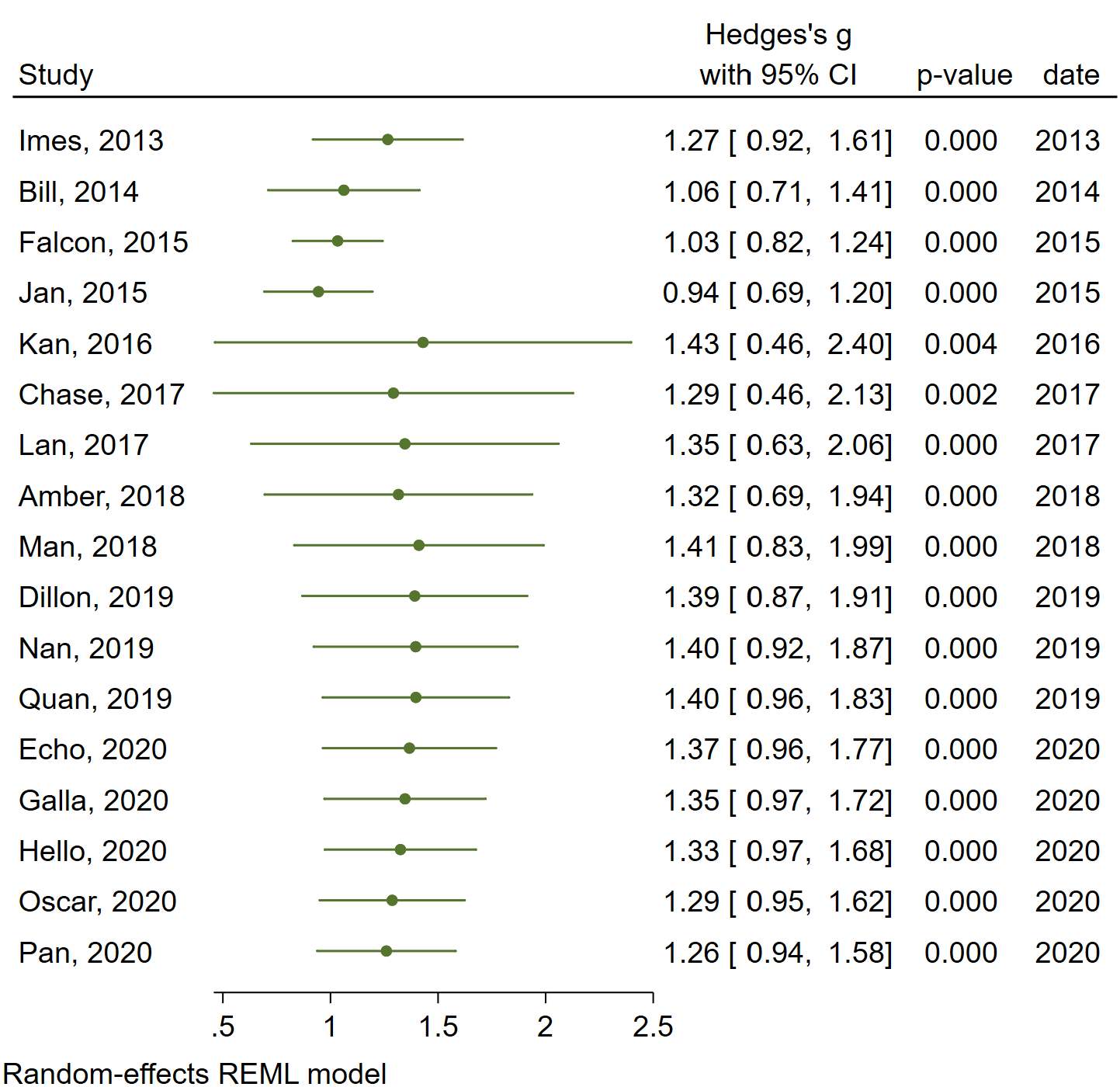
Concluding remarks
Clearly the purpose of the today’s discussion has been to introduce you to the what, why and how of meta-analysis. But I hope that it also makes you think about the reporting of your primary research as well. For example, many researchers conduct an a priori power analysis. When you do so, you need to guess at your effect size. When your study is complete and the data have been analyzed, perhaps you should calculate the effect size (you might need to include this in your paper anyway). Compare your calculated effect size with the guess you made when running the power analysis. How accurate was your guess? If you do this with each of your primary studies, you might find that you tend to under- or overestimate effect sizes when running power analyses. Also, when you report an effect size, be sure to include its standard error. You may also want to include a few more descriptive statistics in your paper, as a future meta-analyst may be looking at something slightly different than you.
Two final points: Try to be responsive to requests for additional information regarding studies that you published. Secondly, make sure that older data and syntax/command/script files are readable with the current technology. For example, I still have ZIP disks. Finding a ZIP drive isn’t that difficult, but finding drivers is a little more challenging. My point is that you need to pay attention to both hardware and software when maintaining older files.
While we have discussed many topics, there are still quite a few that we have not discussed, such as multiple imputation for missing data, multilevel modeling, psychometric meta-analysis, network meta-analysis, SEM, generalized SEM and power analyses. These are more advanced topics that are beyond the scope of an introductory workshop. On a final note, I want to say that the area of meta-analysis is an area of statistics that is evolving and changing rapidly. This means that reviewing the current guidelines regarding the conducting and reporting of a meta-analysis is extra important, even if you have published meta-analyses in the past.
References
Borenstein, M., Hedges, L. V., Higgins, J. P. T., and Rothstein, H. R. (2021). Introduction to Meta-Analysis, Second Edition. Wiley: United Kingdom.
Borenstein, M., Hedges, L. V., Higgins, J. P. T., and Rothstein, H. R. (2009). Introduction to Meta-Analysis. Wiley: United Kingdom.
Borenstein, M. (2019). Common Mistakes in Meta-analysis and How to Avoid Them. Biostat, Inc.: Englewood, New Jersey.
Cleophas, T. J. and Zwinderman, A. H. (2017). Modern Meta-analysis: Reivew and Update of Methodologies. Springer International: Switzerland.
CONSORT: CONsolidated Standards Of Reporting Trials (http://www.consort-statement.org/ and http://www.equator-network.org/reporting-guidelines/consort/ )
Countway Library of Medicine: https://guides.library.harvard.edu/meta-analysis/guides .
Dixon (1953), “Processing Data for Outliers,” Biometrics, Vol. 9, No. 1, pp. 74-89.
Dixon and Massey (1957), “Introduction to Statistical Analysis,” Second Edition, McGraw-Hill, pp. 275-278.
Downs, S. H. and Black, N. (1998). The feasibility of creating a checklist for the assessment of the methodological quality both of randomised and non-randomised studies of health care interventions. Journal of Epidemiological Community Health. Vol. 52, pages 377-384.
Duval, S. and Tweedie, R. (2000). Trim and fill: A simple funnel-plot-based method of testing and adjusting for publication bias in meta-analysis. Biometrics (June). Vol 56(2): 455-463. (https://www.ncbi.nlm.nih.gov/pubmed/10877304 )
Egger, M., Davey-Smith, G. Schneider, M. and Minder C. (1997). Bias in Meta-Analysis Detected by a Simple, Graphical Test. British Medical Journal (Sept. 13) Vol. 315(7109): 629-634. (https://www.ncbi.nlm.nih.gov/pubmed/9310563 )
Grubbs F.E. (1950). Sample criteria for testing outlying observations. Ann. Math. Stat. 21, 27-58.
Grubbs F.E. (1969). Procedures for detecting outlying observations in samples. Technometrics, 11(1), 1-21.
Grubbs, F.E. and Beck G. (1972). Extension of sample sizes and percentage points for significance tests of outlying observations. Technometrics, 14, 847-854.
Hedges, L. V. and Pigott, T. D. (2001). The Power of Statistical Tests in Meta-Analysis. Psychological Methods. Vol 6(3): 203-2017. (https://www.ncbi.nlm.nih.gov/pubmed/11570228 )
MOOSE: Meta-analysis Of Observational Studies in Epidemiology (http://statswrite.eu/pdf/MOOSE%20Statement.pdf and http://www.ijo.in/documents/14MOOSE_SS.pdf )
Orwin, R. G. (1983). A fail-safe N for effect size in meta-analysis. Journal of Educational Statistics. Vol. 8(2) Summer, 1983, 157-159.
Palmer, T. M. and Sterne, J. A. C. (2009). Meta-Analysis in Stata: An Updated Collection from the Stata Journal, Second Edition. Stata Press: College Station, TX.
PRISMA: Preferred Reporting Items for Systematic reviews and Meta-Analyses (http://www.prisma-statement.org/ )
QUOROM: QUality Of Reporting Of Meta-analyses (https://journals.plos.org/plosntds/article/file?type=supplementary&id=info:doi/10.1371/journal.pntd.0000381.s002 )
Rosenthal, R. (1979). The file drawer problem and tolerance for null results: Psychological Bulletin. Vol 86(3) May 1979, 638-641.
Stata blog: https://blog.stata.com/2013/09/05/measures-of-effect-size-in-stata-13/
Sterne, J. A. and Davey-Smith, G. (2001). Sifting the evidence-what’s wrong with significance tests? British Medical Journal (Jan. 27). Vol. 322(7280): 226-231. (https://www.ncbi.nlm.nih.gov/pubmed/11159626 )
STROBE: Strengthening The Reporting of OBservational studies in Epidemiology (https://www.strobe-statement.org/index.php?id=strobe-home and https://www.strobe-statement.org/index.php?id=available-checklists )
https://www.psychometrica.de/effect_size.html .
http://faculty.ucmerced.edu/wshadish/software/es-computer-program
Wikipedia: https://en.wikipedia.org/wiki/Effect_size .