
Introduction
Missing data is a common issue, and more often than
not, we deal with the matter of missing data in an ad hoc fashion.
The purpose of this seminar is to discuss commonly used techniques for handling missing data
and common issues that could arise when these techniques are used. In
particular, we will focus on the one of the most popular methods, multiple imputation. We are not advocating in favor of any one technique to handle missing data
and depending on
the type of data and model you will be using, other techniques such as direct
maximum likelihood may better serve your needs. We have
chosen to explore multiple imputation through an examination of the data, a careful consideration of the
assumptions needed to implement this method and a clear understanding of the
analytic model to be estimated. We hope this seminar will help you to better
understand the scope of the issues you might face when dealing with missing data
using this method.
The
data set
hsb2_mar.dta
which is based on hsb2.
Some of the variables have value labels associated with
them.
Goals of statistical analysis with missing data:
- Minimize bias
- Maximize use of available information
- Obtain appropriate estimates of uncertainty
Exploring missing data mechanisms
The missing data mechanism describes the process that is believed to have generated the missing
values. Missing
data mechanisms generally fall into one of three main categories. There are precise
technical definitions for these terms in the literature; the following
explanation necessarily contains simplifications.
- Missing completely at
random (MCAR)
A variable is missing completely at random, if neither the variables in the
dataset nor the unobserved value of the variable itself predict whether a
value will be missing. Missing completely at random is a fairly strong
assumption and may be relatively rare. One relatively common situation in which
data are missing completely at random occurs when a subset of cases
is randomly selected to undergo additional measurement, this is
sometimes referred to as “planned missing.” For example, in some health
surveys, some subjects are randomly selected to undergo more extensive
physical examination; therefore only a subset of participants will have complete
information for these variables. Missing completely at random also allow for missing on one
variable to be related to missing on another, e.g. var1 is missing whenever var2
is missing. For example, a husband and wife are both missing information on
height.
- Missing at random (MAR)
A variable is said to be missing at random if other variables (but not the
variable itself) in the dataset can be
used to predict missingness on a given variable. For example, in surveys, men may be more likely to decline to answer
some questions than women (i.e., gender predicts missingness on another variable).
MAR is a less restrictive assumption than MCAR. Under this assumption the probability of missingness does not
depend on the true values after controlling for the observed variables. MAR is also related to ignorability. The missing
data mechanism is said be ignorable if it is missing at random
and the
probability of a missingness does not depend on the missing information itself. The assumption of ignorability is needed for optimal estimation of missing
information and is a required assumption for both of the missing data techniques
we will discuss.
- Missing not at random (MNAR)
Finally, data are said to be missing not at random if the value of the
unobserved variable itself predicts missingness. A classic example of this is
income. Individuals with very high incomes are more likely to decline to
answer questions about their income than individuals with more moderate incomes.
An understanding of the missing data mechanism(s) present in your data is
important because different types of
missing data require different treatments. When data are missing completely at
random, analyzing only the complete cases will not result in biased parameter
estimates (e.g., regression coefficients). However, the sample size for an
analysis can be substantially reduced, leading to larger standard errors. In
contrast, analyzing only complete cases for data that are either missing at
random, or missing not at random can lead to biased parameter estimates.
Multiple imputation and other modern methods such as direct maximum likelihood generally assumes that the data are at least MAR, meaning that this procedure can also be used on data that are missing
completely at random. Statistical models have also been developed for modeling
the MNAR processes; however, these model are beyond the scope of this seminar.

For more information on missing data mechanisms please see:
- Allison, 2002
- Enders, 2010
- Little & Rubin, 2002
- Rubin, 1976
- Schafer & Graham, 2002
Full data:
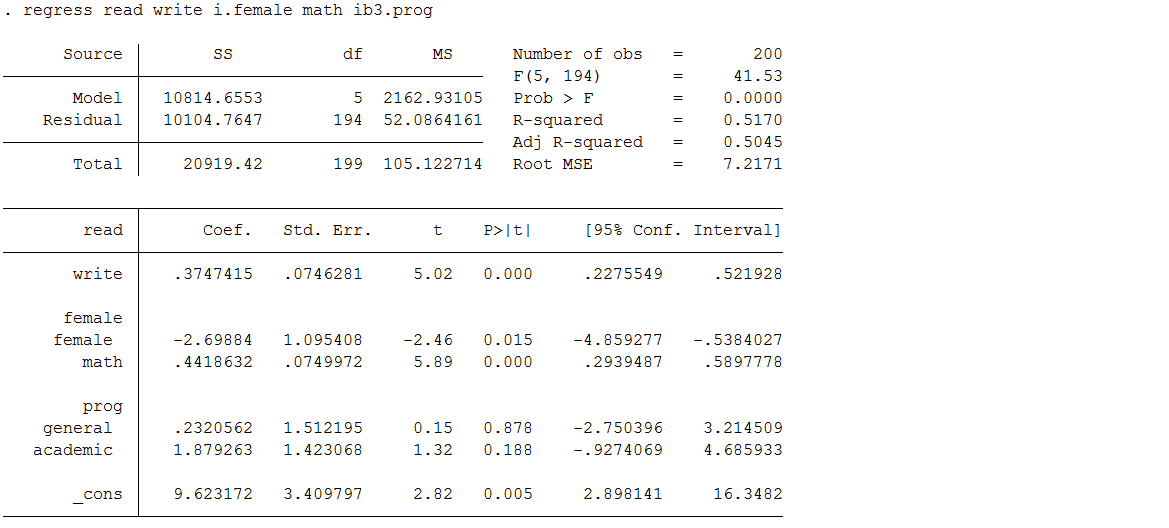
Below is a regression model predicting read using the complete data set (hsb2) used to
create hsb_mar, which contains test scores, as well as
demographic and school information for 200 high school students. We will use these results for comparison.
use https://stats.idre.ucla.edu/stat/stata/notes/hsb2
regress read write i.female math ib3.prog
Common techniques for dealing with missing data
In this section, we are going to discuss some common techniques for
dealing with missing data and briefly discuss their limitations.
- Complete case analysis (listwise deletion)
- Available case analysis (pairwise deletion)
- Mean Imputation
- Single Imputation
- Stochastic Imputation
1. Complete Case Analysis:
This methods involves deleting cases in a particular dataset that are missing
data on any variable of interest. It is a common technique because it is easy to implement
and works with any type of analysis.
Below we look at some of the descriptive statistics of the data set
hsb_mar.
use https://stats.idre.ucla.edu/wp-content/uploads/2017/05/hsb2_mar.dta, clearsum
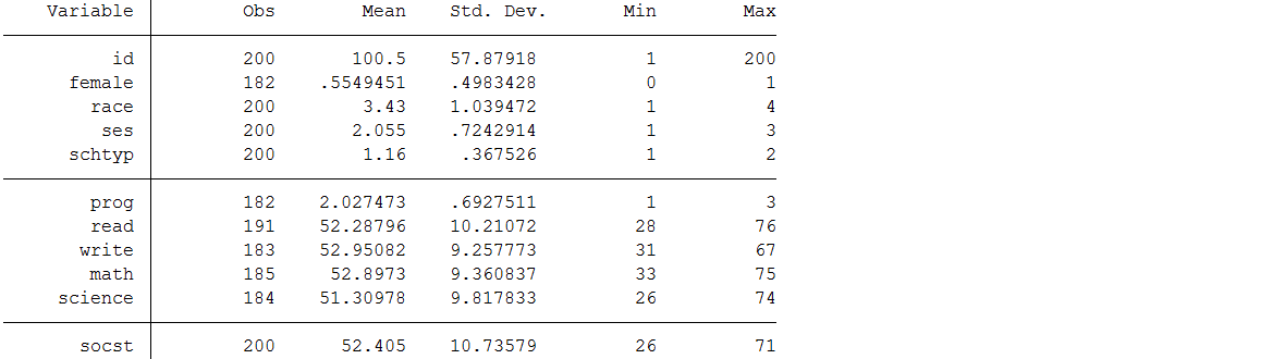
Note that although the dataset contains 200 cases, six of the variables have
fewer than 200 observations. The missing information
varies between 9 observations or 4.5% (read)
and 18 observations or 9% (female
and prog)
of cases
depending on the variable. This doesn’t seem like a lot of
missing data, so we might be inclined to try to analyze the observed data as
they are,
a strategy sometimes referred to as complete case analysis.
Below is a regression model where the dependent variable read is
regressed on
write, math, female and prog. Notice that the default
behavior of the command regress is complete case analysis (also referred to as listwise
deletion).
use https://stats.idre.ucla.edu/wp-content/uploads/2017/05/hsb2_mar.dta, clearregress read write i.female math ib3.prog
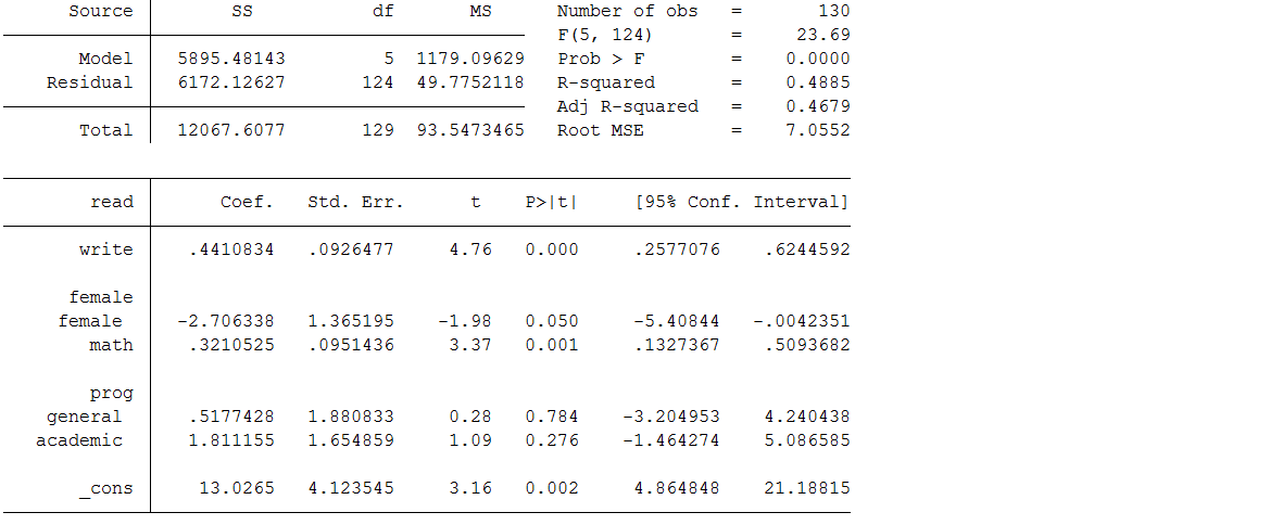
Looking at the output, we see that only 130 cases were used in the
analysis; in other words, more than one third of the cases in our dataset
(70/200) were excluded from the analysis because of missing data. The reduction in sample size
(and statistical power) alone might be considered a problem, but complete case
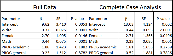
analysis can also lead to biased estimates. Specifically you will see below that the
estimates for the intercept, write, math and prog
are different from the regression model on the complete data. Also, the standard
errors are all larger due to the smaller sample size, resulting in the parameter
estimate for female becoming borderline non-significant. Unfortunately, unless the
mechanism of missing data is MCAR, this method will introduce bias into the
parameter estimates.
2. Available Case Analysis:
This method involves estimating means, variances and covariances based on all
available non-missing cases. Meaning that a covariance (or correlation) matrix
is computed where each element is based on the full set of cases with
non-missing values for each pair of variables. This method became popular
because the loss of power due to missing information is not as substantial as
with complete case analysis. Depending on the pairwise
comparisons examined, the sample size will change based on the amount of missing
present
in one or both variables. One of the main drawbacks of
this method is no consistent sample size and the parameter estimates produced
are often much different than the estimates obtained from analysis on the full
data or the listwise deletion approach. Unless the mechanism of missing data is
MCAR, this method will introduce bias into the parameter estimates. Therefore,
this method is not recommended.
3. Unconditional Mean Imputation:
This methods involves replacing the missing values for an individual variable
with its overall estimated mean from the available cases. While this is a simple
and easily implemented method for dealing with missing values it has some
unfortunate consequences. The most important problem with mean imputation, also
called mean substitution, is that it will result in an artificial reduction in
variability due to the fact you are imputing values at the center of the
variable’s distribution. This also has the unintended consequence of changing
the magnitude of correlations between the imputed variable and other variables. We can
demonstrate this phenomenon in our data.
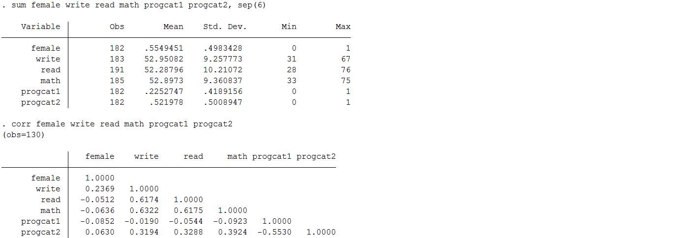
Below are tables of the means and standard deviations of the four variables
in our regression model BEFORE and AFTER a mean imputation as well as their
corresponding
correlation matrices. This will require us to create dummy variables for our
categorical predictor
prog.
tab prog, gen(progcat)
Means and correlations between variables before mean imputation
Means and correlations between variables after mean imputation.
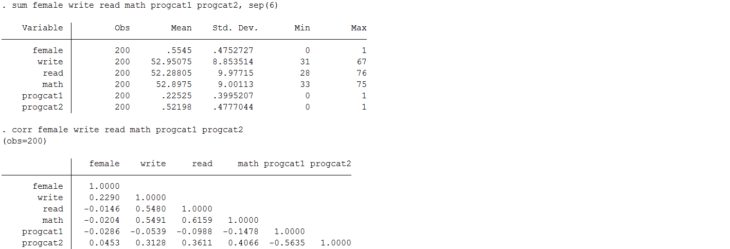
You will notice that there is very little change in the mean (as you
would expect); however, the standard deviation is noticeably lower after
substituting in mean values for the observations with missing information. This
is because you reduce the variability in your variables when you impute everyone
at the
mean. Moreover, you can see the table of correlation
coefficients that the correlation between each of our predictors of interest
( write , math , female , and
prog) as well as between predictors and the
outcome read have now be attenuated. Therefore, regression
models that seek to estimate the associations between these variables will also
see their effects weakened.
4. Single or Deterministic Imputation :
A slightly more sophisticated type of imputation is a regression/conditional
mean imputation, which replaces missing values with predicted scores from
a regression equation. The strength of this approach is that it uses
complete information to impute values. The drawback here is that
all your predicted values will fall
directly on the regression line once again decreasing
variability, just not as much as with unconditional mean imputation.
Moreover, statistical models cannot distinguish between observed and imputed
values and therefore do not incorporate into the model the error or uncertainly
associated with that imputed value. Additionally,
you will see that this method will also inflate the associations between
variables because it imputes values that are perfectly correlated with
one another. Unfortunately, even under the assumption of MCAR, regression
imputation will upwardly bias correlations and R-squared statistics. Further
discussion and an example of deterministic imputation can be found in Craig Enders book “Applied
Missing Data Analysis” (2010).
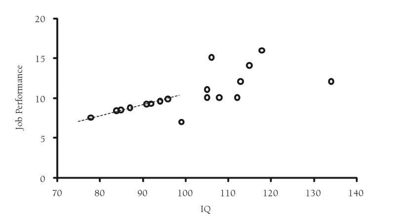
p.46, Applied Missing Data Analysis, Craig Enders (2010)
5. Stochastic Imputation :
In recognition of the problems with regression imputation and the reduced
variability associated with this approach, researchers developed a technique to
incorporate or “add back” lost variability. A residual term, that is randomly
drawn from a normal distribution with mean zero and variance equal to the
residual variance from the regression model, is added to the predicted
scores from the regression imputation thus restoring some of the lost
variability. This method is superior to the previous methods as it will produce unbiased
coefficient estimates under MAR. However, the standard errors produced during
regression estimation while less biased than the single imputation approach, will still
be attenuated.
While you might be inclined to use one of these more traditional methods,
consider this statement: “Missing data analyses are difficult because there is no inherently correct
methodological procedure. In many (if not most) situations, blindly applying
maximum likelihood estimation or multiple imputation will likely lead to a more
accurate set of estimates than using one of the [previously mentioned] missing
data handling techniques” (p.344, Applied Missing Data Analysis, 2010).
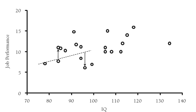
p.48, Applied Missing Data Analysis, Craig Enders (2010)
Multiple Imputation
Multiple imputation is essentially an iterative form of stochastic
imputation. However, instead of filling in a single value, the distribution of
the observed data is used to estimate multiple
values that reflect the uncertainty around the true value. These
values are then used in the analysis of interest, such as in a OLS model, and
the results combined. Each imputed value includes a
random component whose magnitude reflects the extent to which other
variables in the imputation model cannot predict its true values (Johnson and
Young, 2011; White et al, 2010). Thus, building into the imputed values
a level of uncertainty around the “truthfulness” of the imputed values.
A common misconception of missing data methods is the assumption that
imputed values should represent “real” values. The purpose when addressing
missing data is to correctly reproduce the variance/covariance matrix we would
have observed had our data not had any missing information.
MI has three basic phases:
1. Imputation or Fill-in Phase: The missing data are filled in with
estimated values and a
complete data set is created. This process of fill-in is repeated m
times.
2. Analysis Phase: Each of the m complete data sets is then
analyzed using a statistical
method of interest (e.g. linear regression).
3. Pooling Phase: The parameter estimates
(e.g. coefficients and standard errors) obtained from each analyzed data set are then
combined for inference.
The imputation method you choose depends on the pattern of missing
information as well as the type of variable(s) with missing information.
Imputation Model, Analytic Model and Compatibility :
When developing your imputation model, it is important to assess
if your imputation model is “congenial” or consistent with your analytic model. Consistency means that your imputation model includes (at the very least)
the same variables that are in your analytic or estimation model. This
includes any transformations to variables that will be
needed to assess your hypothesis of interest. This can include log transformations, interaction terms, or
recodes of a continuous variable into a categorical form, if that is how it will
be used in later analysis. The reason for this relates back to the earlier
comments about the purpose of multiple imputation. Since we are trying to
reproduce the proper variance/covariance matrix for
estimation, all relationships between our analytic variables should be
represented and estimated
simultaneously. Otherwise, you are imputing
values assuming they have a correlation of zero with the variables you did not
include in your imputation model.
This would result in underestimating the association between parameters of
interest in your analysis and a loss of power to detect properties of your data
that may be of interest such as
non-linearities and statistical interactions. For additional reading on this particular topic see:
1. von Hippel, 2009
2. von Hippel, 2013
3. White et al., 2010
Preparing to conduct MI:
First step: Examine the number and proportion of missing values among your
variables of interest. Let’s reload our dataset and use the mdesc
command to count the number of missing observations and proportion of
missing for each variable.
use https://stats.idre.ucla.edu/wp-content/uploads/2017/05/hsb2_mar.dta, clearmdesc female write read math prog

We can see that the variables with the highest proportion of missing
information are prog and female with 9.0%. In general, you want to note
the variable(s) with a high proportion of missing information as they will have
the greatest impact on the convergence of your specified imputation model.
Second Step: Examine Missing Data Patterns among your variables of interest.
Stata has a suite of multiple imputation (mi) commands to help users
not only impute their data but also explore the patterns of missingness present
in the data.
In order to use these commands the dataset in memory must be declared or
mi set as “mi” dataset. A dataset that is mi set is given an mi style. This
tells Stata how the multiply imputed data is to be stored once the imputation
has been completed. For information on these style type help mi styles
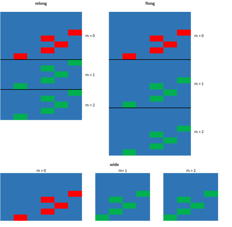
into the command window. We will use the style mlong.
The chosen style can be changed using mi convert.
mi set mlong
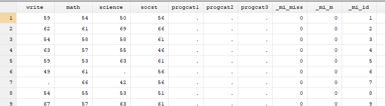
You will notice that executing the previous comand will create three new variables to your dataset.
These new variables will be used by Stata to track the imputed datasets
and values.
- _mi_miss: marks the observations in the original dataset that have
missing values. - _mi_m: indicates the imputation number. The value is 0 for the original
dataset. - _mi_id: indicator for the observations in the original
dataset and is repeated across imputed dataset to mark the imputed
observations.
The mi misstable
commands helps users tabulate the
amount of missing in their variables of interest (summarize) as
well as examine patterns of missing (patterns).
mi misstable summarize female write read math prog

Notice that Stata codes missing values ., .a, .b, .c, …, .z as larger than any nonmissing values:
∞ < . < .a < .b < … < .z
mi misstable patterns female write read math prog
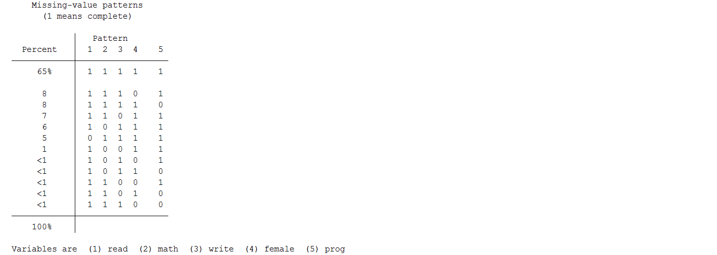
This “Missing-value patterns” table is shown above. Each row represents
a set of observations in the data set that share the same pattern of missing
information. For example, row 1 represents the 65% of observations (n=130) in the data that have complete
information on all 5 variables of interest. You can see that there are a total of 12
patterns for the specified variables. You will want to examine this table for
any patterns and the appearance of any set of variables that appear to always be
missing together. Moreover, depending on the nature of the data, you may also recognize
patterns such as monotone missing which can be observed in longitudinal data
when an individual drops out at a particular time point and therefore all data
after that is subsequently missing. Additionally, you may identify skip patterns
that were missed in your original review of the data that should then be dealt with
before moving forward with the multiple imputation.
Third Step: If necessary, identify potential auxiliary variables
Auxiliary variables are variables in your data set that are either
correlated with a missing variable(s) (the recommendation is r >
0.4) or are believed to be associated with missingness. These are factors that
are not of particular interest in your analytic model , but they are added to
the imputation model to increase power and/or to help make the assumption
of MAR more plausible. These variables have been found to improve the quality of
imputed values generate from multiple imputation. Moreover, research has
demonstrated their particular importance when imputing a dependent variable
and/or when you have variables with a high proportion of missing information (Johnson
and Young, 2011; Young and Johnson, 2010;
Enders , 2010).
You may a priori know of several variables you believe would make good
auxiliary variables based on your knowledge of the data and subject matter. Additionally, a good
review of the literature can often help identify them as well. However, if you are
not sure what variables in the data would be potential candidates (this is often
the case when conducting secondary data analysis), you can uses some
simple methods to help identify potential candidates. One way to identify these variables is by examining associations between
write, read, female, and math with other
variables in the dataset. For
example, let’s take a look at the correlation matrix between our 4 variables of
interest and two other test score variables science and
socst.
tab prog, gen(progcat)
pwcorr female write read math progcat1 progcat2 socst science, obs
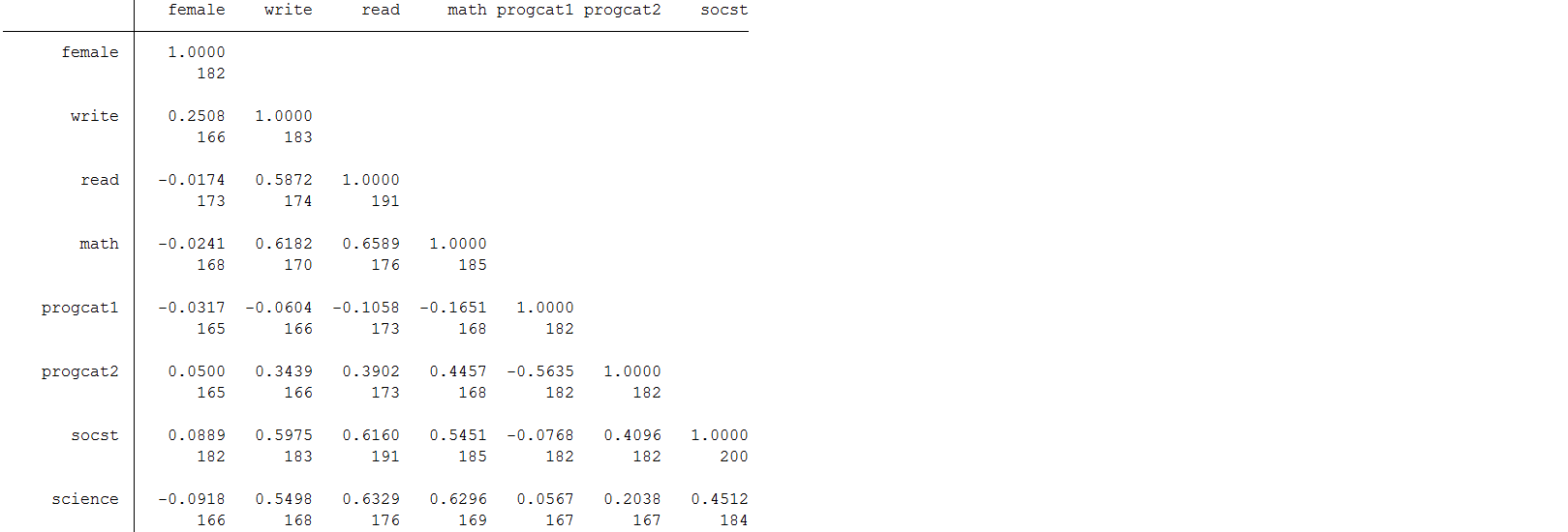
Science and socst both appear to be a good auxiliary because
they are well
correlated (r >0.4) with all the other test score variables of interest. You
will also notice that they are not well correlated with female. A good
auxiliary does not have to be correlated with every variable to be useful. You will also notice that science
also has missing information of its own. Additionally, a good auxiliary is
not required to have complete
information to be valuable. They can have missing and still be effective in reducing bias (Enders, 2010).
One area, this is still under active research, is whether it is beneficial
to include a variable as an auxiliary if it does not pass the 0.4 correlation
threshold with any of the variables to be imputed. Some researchers believe that including
these types of items introduces unnecessary error into the imputation model (Allison, 2012),
while others do not
believe that there is any harm in this practice (Ender, 2010). Thus. we leave it up to you as the researcher to use your
best judgment.
Good auxiliary variables can also be correlates or
predictors of missingness. Let’s create a set of missing data flags for each
variable to be imputed. We will then examine if our
potential auxiliary variable socst also appears to predict
missingness.
gen female_flag=1
replace female_flag=0 if female==.

gen write_flag=1
replace write_flag=0 if write==.

gen read_flag=1
replace read_flag=0 if read==.

gen math_flag=1
replace math_flag=0 if math==.

gen prog_flag=1
replace prog_flag=0 if prog==.
Below are a set of t-tests to test if the mean socst
or science scores differ significantly between those with missing
information and those
without.
foreach var of varlist female_flag - prog_flag{
display "`var'"
ttest socst, by(`var')
}

foreach var of varlist female_flag - prog_flag{
display "`var'"
ttest science, by(`var')
}
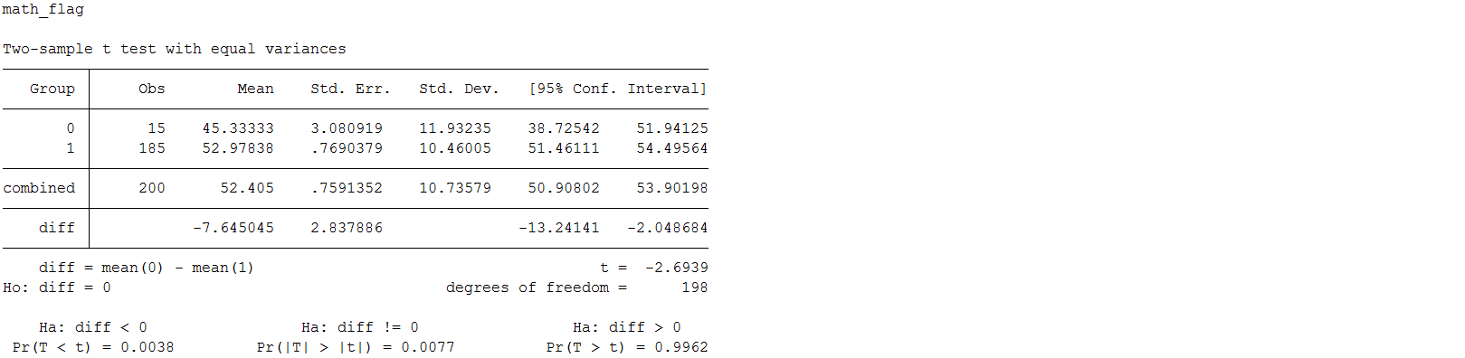
The only significant difference was found when examining missingness on
math with socst. Above you can see that the mean socst score is significantly
lower among the respondents who are missing on math. This
suggests that socst is a potential correlate of missingness
(Enders,
2010) and may help us satisfy the MAR assumption for
multiple imputation by including it in our imputation model.
Example 1: MI using multivariate normal distribution (MVN):
Upon choosing to impute one or many variables, one of the first decisions
you will make is the type of distribution under which you want
to impute your variable(s). One available method uses Markov Chain Monte Carlo (MCMC)
procedures which assume that all the variables in the imputation model have a
joint multivariate normal distribution. This is probably the most common
parametric approach for multiple imputation. The specific algorithm used
is
called the data augmentation
(DA) algorithm, which belongs to the family of
MCMC procedures. The algorithm fills in missing data by
drawing from a conditional distribution, in this case a multivariate normal, of
the missing data given the observed data. In most cases, simulation studies have
shown that assuming a MVN distribution leads to reliable estimates even when the
normality assumption is violated given a sufficient sample size (Demirtas et al., 2008; KJ Lee, 2010). However, biased estimates have been observed when the
sample size is relatively small and the fraction of missing information is high.
Note: Since we are using a multivariate normal distribution for imputation,
decimal and negative values are possible. These values are not a problem for
estimation; however, we will need to create dummy variables for the nominal
categorical variables so the parameter estimates for each level can be
interpreted.
1. Imputation Phase:
After the data is mi set, Stata requires 3 additional
commands. The first is mi register imputed. This command identifies which variables in the imputation model have missing information.
mi register imputed female write read math progcat1 progcat2 science
The second
command is mi impute mvn
where the user specifies the imputation model to be used and the number of
imputed datasets to be created.
mi impute mvn female write read math progcat1 progcat2 science = socst, add(10) rseed (53421)
On the mi impute mvn
command line we can use the add option to specify the number of imputations to be performed.
In this example we chose 10 imputations. Variables on the left side of the
equal sign have missing information, while the right side is reserved for
variables with no missing information and are therefore solely considered
“predictors” of missing values. As you can see, even through
science is an auxiliary variable, science must be
included as a variable to be imputed.
After the
mvn all the variables for the imputation model are specified including
all the variables in the analytic model as well as any auxiliary variables. The
option rseed is not required, but since MI is designed to be a
random process, setting a seed will allow you to obtain the same imputed dataset
each time. The imputed datasets will be stored appended or “stacked” together in a dataset.
The
indicator variable called _mi_m is automatically populated to
number each new imputed dataset (1 -10).
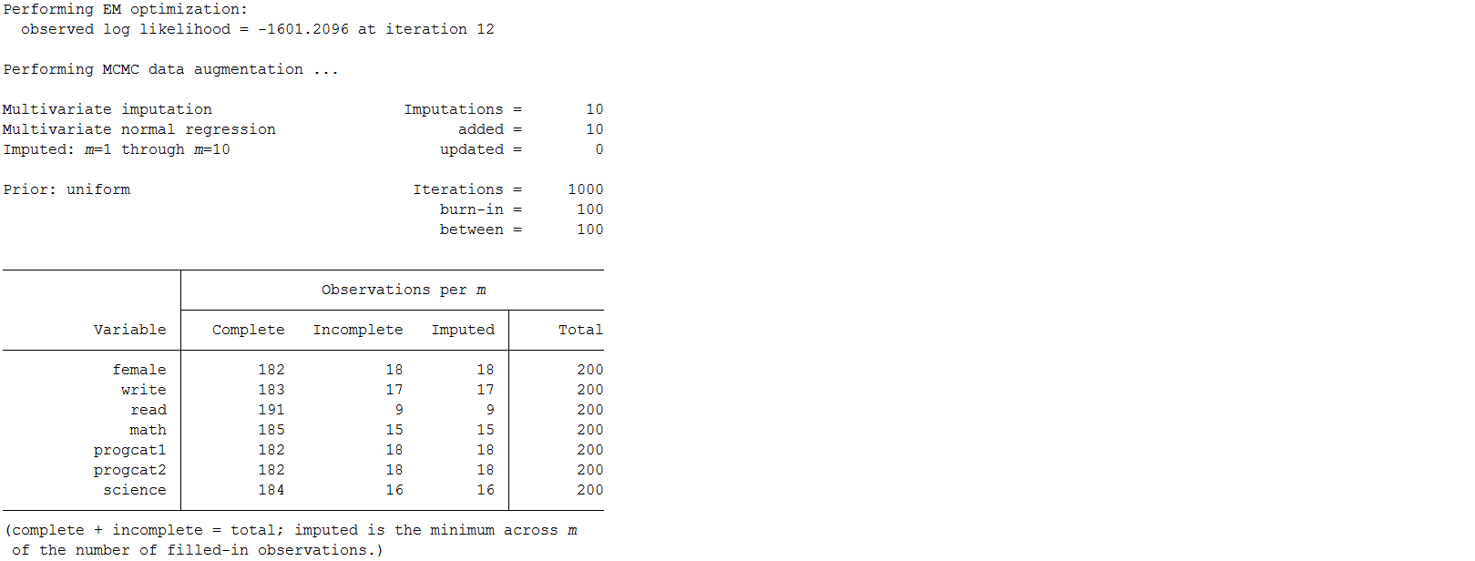
The output after mi impute mvn, let’s the user know what
options have been invoked for the command. The top of the output shows what
type of imputation was used (MVN), as well as the number of imputed data sets
created (m=10). Because the estimation of the imputed values involves a Bayesian
process, characteristics of the MCMC are also reported, including the type of
prior used, the total number of iterations, the number of burn-in iterations (number
of iterations before the first set of imputed values is drawn) and the number of
iterations between draws. The bottom portion of the output includes a table that
reports
the number of missing values that were imputed for each variable that was
registered to be imputed.
2. Analysis/Pooling Phase:
The third step is mi estimate
which runs the analytic model of
interest (here it is a linear regression using regress) within
each of the imputed datasets. It also combines all the estimates
(coefficients and standard errors) across all the imputed datasets.
The mi estimate command is used as a prefix to the standard
regress command. This executes the specified estimation model
within each of the 10 imputed datasets to obtain 10 sets of coefficients and
standard errors. Stata then combines these estimates to obtain one set of inferential
statistics.
mi estimate: regress read write female math progcat1 progcat2

This step combines the parameter estimates into a single set of statistics
that appropriately reflect the uncertainty associated with the imputed values.
The regression coefficients are simply just an arithmetic mean of the individual
coefficients estimated for each of the 10 regression models. Averaging the
parameter estimates dampens the variation thus increasing efficiency and
decreasing sampling variation. Estimation of the standard error for each
variable is little more complicated and will be discussed in the next section.
If you compare these estimates to those from the complete data you will observe
that they are, in general, quite comparable. The variables write, female and math,
are significant in both sets of data. You will also observe a small inflation in
the standard errors, which is to be expected since the multiple imputation
process is designed to build additional uncertainty into our estimates.
| Full Data | Complete Case | MVN Imputation | |||||||||
| Parameter | β | SE | P-value | Parameter | β | SE | P-value | Parameter | β | SE | P-value |
| Intercept | 9.62 | 3.410 | 0.0053 | Intercept | 13.03 | 4.124 | 0.002 | Intercept | 10.35 | 3.687 | 0.006 |
| Write | 0.37 | 0.075 | <.0001 | Write | 0.44 | 0.093 | <.0001 | Write | 0.39 | 0.082 | <.0001 |
| Female | -2.70 | 1.095 | 0.0146 | Female | -2.71 | 1.365 | 0.0496 | Female | -2.74 | 1.144 | 0.017 |
| Math | 0.44 | 0.075 | <.0001 | Math | 0.32 | 0.095 | 0.001 | Math | 0.40 | 0.087 | <.0001 |
| PROG academic |
1.88 | 1.423 | 0.1882 | PROG academic | 1.81 | 1.655 | 0.2759 | PROG academic | 2.81 | 1.602 | 0.083 |
| PROG general | 0.23 | 1.512 | 0.8782 | PROG general | 0.52 | 1.881 | 0.7836 | PROG general | 0.52 | 1.685 | 0.76 |
2. Imputation Diagnostics:
In the output from mi estimate you will see several metrics
in the upper right hand corner that you may find unfamilar These
parameters are estimated as part of the imputation and allow the user to assess how well the imputation
performed. By
default, Stata provides summaries and averages of these values but the
individual estimates can be obtained using the vartable and
dftable options.
Let’s take a look at the information for RVI (Relative Increase in Variance), FMI
(Fraction of Missing Information), DF (Degrees of Freedom) , RE (Relative
Efficiency), as well as the between imputation and the within imputation
variance estimates to examine how the standard errors (SEs) are calculated.
mi estimate, vartable dftable
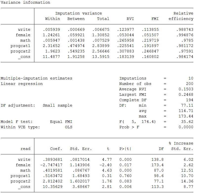
Below we discuss each piece:
- Variance Between (VB):
- This is a measure of the variability in the parameter estimates
(coefficients) obtained from the 10 imputed datasets- For example, if you took all 10 of the
parameter estimates for write
and calculated
the variance this would equal VB =
0.00067.
- For example, if you took all 10 of the
- This variability estimates the additional variation (uncertainty)
that results from missing data.
- This is a measure of the variability in the parameter estimates
- Variance Within (VW):
- This is simply the arithmetic mean of the sampling
variances (SE) from each of the 10 imputed datasets.- For example, if
you squared the standard errors for
write
for all 10 imputations and then divided by 10, this would equal Vw
= 0.0059
- For example, if
- This estimates the sampling variability that we would have expected
had there been no missing data.
- Variance Total (VT):
-
- The primary usefulness of MI comes from how the total variance is
estimated. - The total variance is sum of multiple
sources of variance. - While regression coefficients are just averaged across imputations,
Rubin’s formula (Rubin, 1987) partitions
variance into “within imputation” capturing the expected
uncertainty and “between imputation” capturing the
estimation variability due to missing information
(Graham, 2007; White et al., 2010). - The total variance is the sum of 3 sources
of variance. The within, the between and an
additional source of sampling variance.- For example, the
total variance for the variable write would be
calculated like this: VB
+ Vw
+ VB/m
= 0.00067
+ 0.0059 + 0.00067/10 = 0.00667
- For example, the
- The additional sampling variance is literally the
variance between divided by m.
This value represents the sampling error associated with the overall or
average coefficient estimates. It is used as a correction factor for
using a specific number of imputations.
- This value becomes smaller, the more imputations are conducted. The
idea being that the larger the number of imputations, the more precise
the parameter estimates will be.
- This value becomes smaller, the more imputations are conducted. The
- Bottom line: The main difference between multiple
imputation and other single imputation methods, is in the estimation of
the variances. The SEs for each parameter estimate are the square root of their VT s
- The primary usefulness of MI comes from how the total variance is
-
- Relative Increases in Variance (RIV/RVI):
- Proportional increase in total sampling variance that is due to
missing information ([VB + VB/m]/VW). - For example, the RVI
for write is 0.1239 this means that the estimated sampling
variance for write is 12.4% larger than its sampling
variance would have been had the data on write been complete. - Bottom line: Variables with large amounts of missing
and/or that are weakly correlated with other variables in the imputation
model will tend to have high RVI’s.
- Proportional increase in total sampling variance that is due to
- Fraction of Missing Information (FMI):
- Is directly related to RVI.
- Proportion of the total sampling variance that is due to missing data ([VB+
VB/m
]/VT)
. - It’s estimated based on the percentage missing for a particular
variable and how correlated this variable is with other variables in the
imputation model. - The interpretation is similar to an R-squared. So an FMI of 0.1138 for
write means that 11.4% of the total
sampling variance is attributable to missing data. - The accuracy of the estimate of
FMI increases as the number imputation increases because variance
estimates stabalize with larger numbers imputations. This especially
important in the presence of a variable(s) with a high proportion of
missing information. - If convergence of your imputation
model is slow, examine the FMI estimates for each variables in your
imputation model. A high FMI can indicate a problematic variable. - Bottom line: If FMI is high for any particular
variable(s) then consider increasing the number of imputations. A good
rule of thumb is to have the number imputations (at least) equal the highest FMI
percentage.
- Relative Efficiency:
- The relative (variance) efficiency (RE) of an imputation (how well the true population
parameters are estimated) is related to both the amount of
missing information as well as the number (m) of imputations performed. - RE is an estimate of the effficiency relative to performing an
infinite number of imputations. - When the amount of missing information is very low then efficiency
may be achieved by only performing a few imputations (the minimum number given in most of the
literature is 5). However when there is high amount of missing information, more
imputations are typically necessary to achieve adequate efficiency for parameter
estimates. You can obtain relatively good efficiency even with a small
number of m. However, this does not mean that the standard errors will
be well estimated well. - More imputations are often necessary for proper standard error
estimation as the variability between imputed datasets incorporate the
necessary amount of uncertainty around the imputed values. - The direct relationship
between RE, m and the FMI is:
1/(1+FMI/m).
This formula represent the RE of
using m imputation versus the infinte number of imputations. To get an idea of what this looks
like practically, take a look at an example from
SAS
documentation. - Bottom line: It may appear that you can get good RE
with a few imputations; however, it often takes more imputations to get
good estimates of the variances than good estimates of parameters like
means or regression coefficients.
- The relative (variance) efficiency (RE) of an imputation (how well the true population
- Degrees of Freedom (DF):
- Unlike analysis with non-imputed data, sample size does not directly
influence the estimate of DF. - DF actually continues to increase as the number of imputations
increase. - The standard formula used to calculate DF can result in fractional
estimates and inflated degrees of freedom. - A small-sample correction to the DF (Barnard and Rubin, 1999)
is implemented (by default) in order to
address the inflated DF the can sometimes occur when the number of
m is large. - Bottom line:
The
standard uncorrected formula assumes that the estimator has a normal
distribution, i.e. a t-distribution with infinite degrees of freedom. In
large samples this is not usually an issue but can be with smaller sample
sizes. In that case, the default corrected formula should be used (Lipsitz et
al., 2002).
- Unlike analysis with non-imputed data, sample size does not directly
After performing an imputation it is also useful to look at means,
frequencies and box plots comparing observed and imputed values to assess
if the range appears reasonable. You may also want to examine plots of residuals
and outliers for each imputed dataset
individually. If anomalies are evident in only a small number of
imputations then this indicates a problem with the imputation model (White et al, 2010).
You should also assess convergence of your imputation model. This
should be done for different imputed variables, but specifically for those variables
with a high proportion of missing (e.g. high FMI).
Convergence of the imputation model means that DA algorithm has reached an
appropriate stationary posterior distribution. Convergence for each imputed
variable can be assessed using trace plots. Trace plots are plots of estimated
parameters against iteration numbers. These plots can be
requested using the
saveptrace
and mcmconly option.
This mcmconly option will simply
run the MCMC algorithm for the same number of iterations it takes to obtain 10
imputations without actually producing 10 imputed datasets. Is it typically used in
combination with saveptrace or savewlf to
examine the convergence of the MCMC prior to imputation. No imputation is
performed with mcmconly is specified, so the options
add or replace are not required with mi
impute mvn.
In practice, convergence is often examined visually from the trace and
autocorrelation plots of the estimated parameters. Trace plots are plots of
estimated parameters against iteration numbers. Long-term trends in trace plots
and high serial dependence in autocorrelation plots are indicative of a slow
convergence to stationarity. A stationary process has a
mean and variance that do not change over time (StataCorp,2017 – Stata 15 “MI
Impute Chained”). You can take a look at examples of
good and bad trace plots in the SAS users guide section on “Assessing
Markov Chain Convergence“.
mi impute mvn write read female math science progcat1 progcat2 = socst,
mcmconly burnin(1000) rseed(53421) saveptrace(trace, replace)
Note that the trace file that is saved is not a true Stata dataset, but it
can be loaded as if they were using the mi ptrace use command
and its contents can be described without actually opening the file using the
command mi ptrace describe. The trace file contains information
on imputation number, iteration number, regression coefficients, variances and
covariances.
mi ptrace describe trace
mi ptrace use trace, clear

If you have a lot of parameters in your model it may not be feasible to
examine the convergence of each individual parameter. In that case you can use
savewlf. WLF stands for worst linear function. This will output to you
the parameter(s) with the highest FMI value.
Let’s take a look at the data for female (y3), which was one of the variables
that contain the fewest number of complete observations. We will generate graphs
for each series.
We will start by declaring the data as time series, so iteration number will be on the x-axis.
We will then graph the regression coefficients and variance for female.
tsset itertsline b_y3x1, name(gr1,replace) ytitle("Coefficient on Socst" "used to predict Female") xtitle("iter") tsline v_y3y3, name(gr2,replace) ytitle(Female Variance) xtitle("iter") graph combine gr1 gr2 , xcommon cols(1) b1title(Iteration)
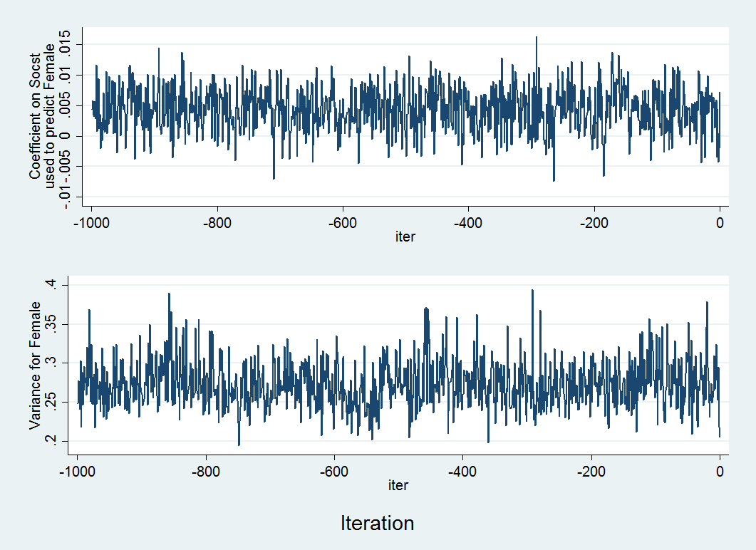
Above is an example of two trace plots. There are two main things you want to note in a trace plot.
First, assess whether the algorithm appeared to reach a stable
posterior distribution by examining the plot to see if the predicted values remains relatively
constant and that there appears to be an absence of any sort of trend
(indicating a sufficient amount of randomness in the coefficients, covariances
and/or variances between iterations). In our case, this looks
to be true. Second, you want to examine the plot to see how long it takes to
reach this stationary phase. In the above example it looks to happen almost
immediately, as no observable pattern emerges, indicating good convergence. By default the burn-in period (number of
iterations before the first set of imputed values is drawn) is 100. This can be increased
if it appears that proper convergence is not achieved using the burnin
option.
Another plot that is very useful for assessing convergence is the auto
correlation plot. Autocorrelation measures the correlation between predicted
values at each iteration. As the imputation process os designed to be random, we
should not observe correlated imputed values across imputations. We can check to see that enough iterations were left
between successive draws (i.e., datasets) that autocorrelation does not exist.
Let’s say you noticed a trend in the variances in the
previous trace plot. You may want to assess the magnitude of the observed
dependency of values across iterations. The auto correlation plot will show you
that. To produce these plots in Stata,
you will use the ac or autocorrelation command on the same
“trace” datafile.
ac b_y3x1, ytitle("Coefficient on Socst" "used to predict Female") xtitle("") ciopts(astyle(none)) ///note("") name(ac1, replace) lags(100)ac v_y3y3, ytitle(Female Variance) xtitle("") ciopts(astyle(none)) note("") name(ac2, replace) lags(100)graph combine ac1 ac2, xcommon cols(1) title(Autocorrelations) b1title(Lag)
In the graph below, the x-axis shows the lag, that is the distance between a
given iteration and the iteration it is being correlated with, on the y-axis is
the value of the correlations. In the plot you can see
that the correlation is high when the mcmc algorithm starts but quickly goes
to near zero after a few iterations indicating almost no correlation between
iterations and therefore no correlation between values in adjacent imputed
datasets. By default Stata, draws an imputed dataset every 100 iterations, if
correlation appears high for more than that, you will need to increase the
number of iterations between imputed datasets using the
burnbetween option. Take a look at the Stata 15 mi impute mvn
documentation for more information about this and other options.
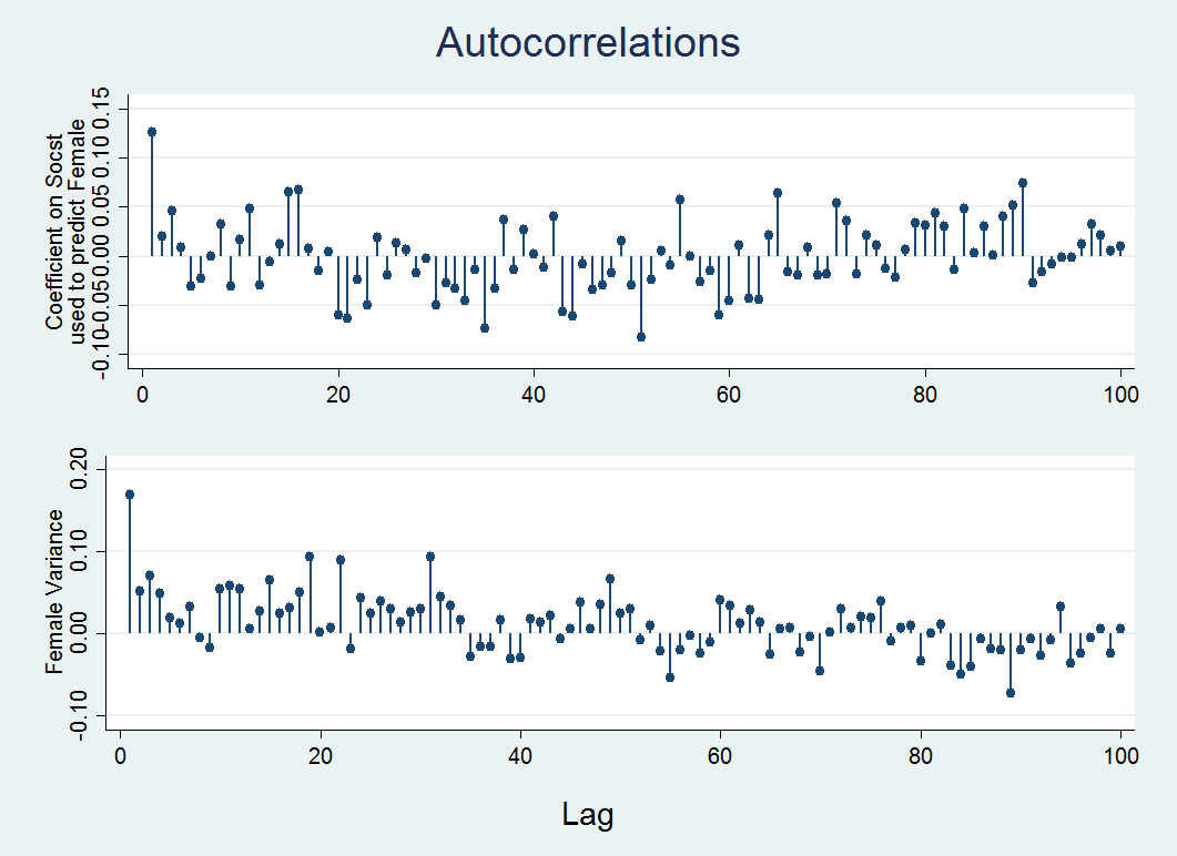
Note: The amount of time it takes to get to zero (or near zero) correlation is an
indication of convergence time (Enders, 2010).
For more information on these and other diagnostic tools, please see Ender, 2010 and
Rubin, 1987.
Example 2: MI using chained equations/MICE (also known as the fully
conditional specification or
sequential generalized regression)
A second method available in Stata is multiple imputation by chained
equations (MICE) which does not assume a joint MVN distribution but instead
uses a separate conditional distribution for each
imputed variable. This specification may be necessary if you are are imputing a
variable that must only take on specific values such as a binary outcome for a
logistic model or a count variable for a Poisson model. In simulation studies (Lee
& Carlin, 2010; Van Buuren, 2007), MICE has been show to produce estimates that
are comparable to MVN method. Later we will discuss some diagnostic tools that
can be used to assess if convergence was reached when using MICE.
The MICE distributions available is Stata are binary, ordered and multinomial logistic
regression for categorical variables, linear regression
and predictive mean matching (PMM)* for continuous variables, and Poisson and negative binomial regression
for count variables. Stata also provides access to some more specialized
methods including truncated and interval regression. If you do not specify a
distribution, by default,
linear regression is used.
For more information on these methods and the options associated with them,
see Stata help file
on the
mi impute chained.
*Note: The default Stata behavior for PMM uses too few
nearest neighbor matches and will reuslt sin underestimated stanrds erros, this
option should be changed when using the procedure.
Let’s reload the data and mi set:
use https://stats.idre.ucla.edu/wp-content/uploads/2017/05/hsb2_mar.dta, clear

mi set mlong
1. Imputation Phase:
The basic set-up for conducting an imputation is shown below. The syntax
look very similar to the previous model using MVN with a few differences. First, we are now
specifying chained instead of mvn.
Second, instead of just listing the variable(s) to be imputed, we will now specify
a particular distribution to impute under. The chosen imputation method is listed
with parentheses directly preceding the variable(s) to which this distribution
applies. In this case, we will use logistic for the binary variable
female, multinomial logistic for our
unordered categorical variable prog, and linear regression for
all of our continuous score variables. You will notice that we no longer
need dummy variables for prog since we are imputing it as a
categorical variable.
mi register imputed female write read math prog science

mi impute chained (logit) female (mlogit) prog (regress) write read math science = socst, ///
add(10) rseed (53421) savetrace(trace1,replace)
By default, the variables will be imputed in order from the most observed to
the least observed. If you would like to override that default, specify the
option orderasis.
As was the case with MVN, Stata will automatically create the variables
_mi_m,_mi_id, _mi_miss.
2. Analysis Phase
Once the 10 multiply imputed datasets have been created, we can run our
linear regression using the regress command. Since we imputed
female and prog under a distribution appropriate for
categorical outcomes, the imputed values will now be true integer values and can
be treated as indicator variables in a regression model.
mi estimate: regress read write i.female math i.prog
As before, the mi estimate command is used as a prefix to the standard
regress command. This executes the specified estimation model
on each of the 10 imputed datasets to obtain 10 sets of coefficients and
standard errors. Stata then combines these estimates to obtain one set of inferential
statistics.
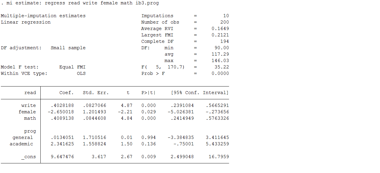
If you compare these estimates to those from the complete data you will
observe that they are, in general, quite comparable. The variables write, female and math,
are significant in both sets of data. You will also observe a small inflation in
the standard errors, which is to be expected since the multiple imputation
process is designed to build additional uncertainty into our estimates. As with
the MVN model, the SE are larger due to the incorporation of uncertainty around
the parameter estimates, but these SE are still smaller than we observed in the
complete cases analysis. The parameter estimates all look good except for those
for prog.
| Full Data | Complete Case | MICE | |||||||||
| Parameter | β | SE | P-value | Parameter | β | SE | P-value | Parameter | β | SE | P-value |
| Intercept | 9.62 | 3.410 | 0.0053 | Intercept | 13.03 | 4.124 | 0.002 | Intercept | 9.65 | 3.620 | 0.009 |
| Write | 0.37 | 0.075 | <.0001 | Write | 0.44 | 0.093 | <.0001 | Write | 0.40 | 0.083 | <.0001 |
| Female | -2.70 | 1.095 | 0.0146 | Female | -2.71 | 1.365 | 0.0496 | Female | -2.65 | 1.201 | 0.029 |
| Math | 0.44 | 0.075 | <.0001 | Math | 0.32 | 0.095 | 0.001 | Math | 0.41 | 0.084 | <.0001 |
| PROG academic |
1.88 | 1.423 | 0.1882 | PROG academic | 1.81 | 1.655 | 0.2759 | PROG academic | 2.34 | 1.559 | 0.136 |
| PROG general | 0.23 | 1.512 | 0.8782 | PROG general | 0.52 | 1.881 | 0.7836 | PROG general | 0.01 | 1.711 | 0.994 |
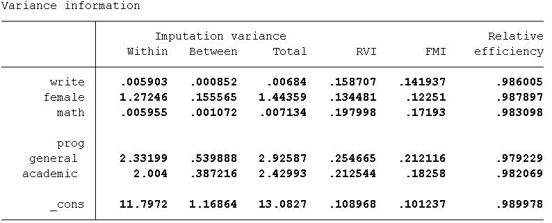
Take a look at some of our imputation diagnostic measures and plots to assess
if anything needs to be changed about our imputation model. Let’s again examine the RVI, FMI, DF, RE as well as the between imputation and the within imputation
variance estimates. As can be seen in the table below, the highest estimated RVI
(25%) and FMI (21%) are associated with
prog. This indicates
that the imputation could potentially be improved by increasing the number of
imputations to 20 or 25 as well as including an auxiliary variable(s) associated with
prog.
As with the MVN method, we can save a file of the predicted values from each
iteration and graph them using a trace plot. The option savetrace
specifies Stata to save the means and standard deviations of imputed values from
each iteration to a Stata dataset named “trace1”.
Note: When using MVN the option is saveptrace.
use trace1,clear

describe
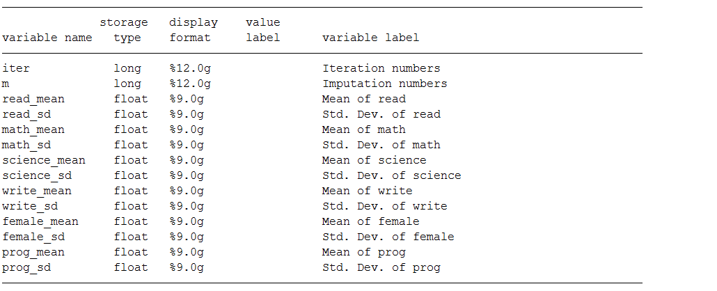
Some data management is
necessary in order to create the trace plot. The file produced by Stata is
“long” with a row for each chain at each iteration. We want the date “wide” so
that the value of mean and standard deviation for each variable are separate by
chain. Since there are multiple chains (m=10), iteration number is repeated which is not
allowed for time series data. Thus, we need to reshape the data beifre we can
use tsset.
Then we can graph the predict mean and/or standard deviation for each imputed
variable.
reshape wide *mean *sd, i(iter) j(m)
tsset iter
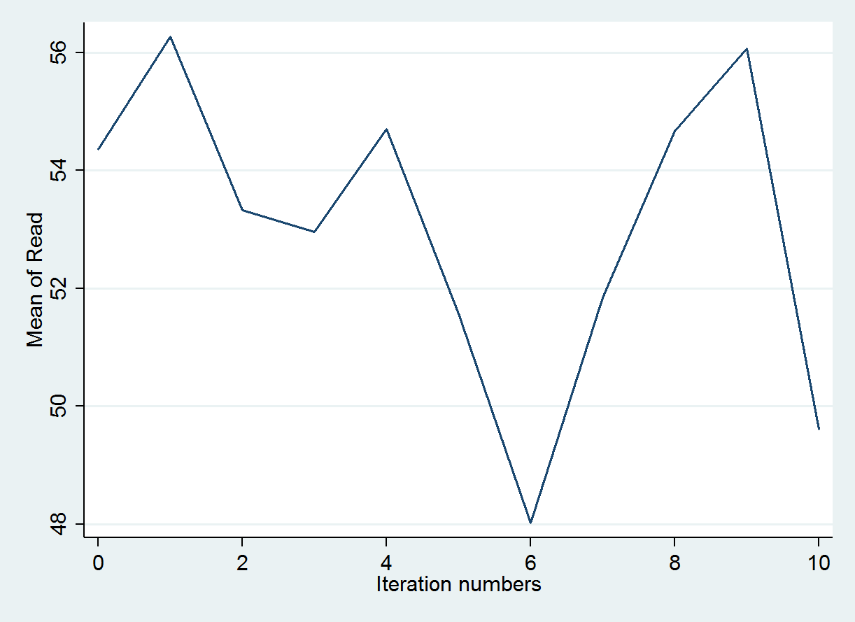
tsline read_mean1, name(mice1,replace)legend(off) ytitle("Mean of Read")
The trace plot below graphs the predicted means value produced during the
first imputation chain. As before, the expectations is that the values
would vary randomly to incorporate variation into the predicted values for
read.
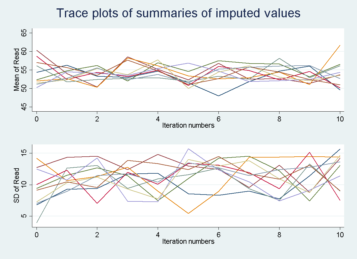
All 10 imputation chains can also be graphed simultaneously to make sure
that nothing unexpected occurred in a single chain. Every chain is obtained
using a different set of initial values and this should be unique. Each colored line
represents a different imputation. So all 10 imputation chains are overlaid
on top of one another.
tsline read_mean*, name(mice1,replace)legend(off) ytitle("Mean of Read")
tsline read_sd*, name(mice2, replace) legend(off) ytitle("SD of Read")
graph combine mice1 mice2, xcommon cols(1) title(Trace plots of summaries of imputed values)
Autocorrelation plots are only available when asuming a joint MVN. In the
case of MICE it would have little usefulness due to the
iterative process used to create the imputations. In each iteration, the
imputation model is estimated using both the observed data and imputed data from
the previous iteration. Thus, you will always get a certain amount of
autocorrelation. For more information on assessing convergence when using
MICE check out Stata’s documentation on mi impute
chained.
MICE has several
properties that make it an attractive alternative to the DA
algorithm. First, the MICE allows each variable to be
imputed using its own conditional distribution instead of one common
multivariate distribution. This especially useful when negative or non-integer
values can not be used in subsequent analyses such as imputing a binary outcome
variable. Second, different imputation models can be specified for different
variables. This is useful if there are particular properties of the data that
need to be preserved. However, the flexibility of the approach can also cause
estimation problems. Specifying different distributions can lead to slow
convergence or non-convergence of the imputation model (See the “Compatability
of Conditionals” and “Convergence of MICE” sections in the Stata help file on
mi impute chained). Additionally, issues of
complete and quasi-complete separation can happen when attempting to impute a
large number of categorical variables. Overall, when attempting multiple
imputation especially with MICE you should allow yourself
sufficient time to build an appropriate model and time for modifications should
convergence and/or estimation problems occur with your imputation model.
The goal is to only have to go through this process once!
Other issues
1. Why Auxiliary variables?
So one question you may be asking yourself, is why are
auxiliary variables necessary or even important. First, they can help
improve the likelihood of meeting the MAR assumption (White
et al, 2011; Johnson and Young, 2011; Allison, 2012). Remember, a variable is said to be missing at random if
other variables in the dataset can be used to predict missingness on a given
variable. So you want your imputation model to include all the variables you
think are associated with or predict missingness in your variable in order to
fulfill the assumption of MAR. Second, including auxiliaries has been shown to
help yield more accurate and stable estimates and thus reduce the estimated
standard errors in analytic models (Enders, 2010; Allison, 2012; von Hippel and
Lynch, 2013). This is especially true in the case of missing outcome variables. Third, including these variable
can also help to increase power (Reis and Judd, 2000; Enders, 2010). In
general, there is almost always a benefit to adopting a more “inclusive analysis
strategy” (Enders, 2010; Allison, 2012).
2. Selecting the number of imputations (m)
Historically, the
recommendation was for three to five MI datasets. Relatively low values of m may
still be appropriate when the fraction of missing information is low and the analysis
techniques are relatively simple. Recently, however, larger values of m
are often being recommended. To some extent, this change in the recommended
number of imputations is based on the radical increase in the computing power
available to the typical researcher, making it more practical to run, create and
analyze multiply imputed
datasets with a larger number of imputations. Recommendations for the number of
m vary. For example, five to twenty imputations for low fractions of missing
information, and as many as 50 (or more) imputations when the proportion of
missing data is relatively high. Remember that estimates of coefficients stabilize
at much lower values of m than estimates of variances and covariances of error
terms (i.e., standard errors). Thus, in order to get appropriate estimates of
these parameters, you may need to increase the m. A larger number of imputations may also allow
hypothesis tests with less restrictive assumptions (i.e., that do not assume
equal fractions of missing information for all coefficients). Multiple runs of
m
imputations are recommended to assess the stability of the parameter estimates.
Graham et al., 2007 conducted a simulation demonstrating the affect on power, efficiency and parameter estimates across
different fractions of missing information as you decrease m. The
authors found that:
1. Mean square error and standard error increased.
2. Power was reduced, especially when FMI is greater than 50% and the
effect size is small, even for a large
number of m (20 or more).
3. Variability of the estimate of FMI increased substantially. In
general , the estimation of FMI improves with an increased m.
4. RE decreased.
Another factor to consider is the importance of reproducibility between
analyses using the same data. White et al. (2010), assuming the true FMI for any
variable would be less than or equal to the percentage of cases that are
incomplete, uses the rule that m should equal the percentage of incomplete
cases. Thus if the FMI for a variable is 20% then you need 20 imputed datasets. A similar analysis by
Bodner, 2008 makes a similar recommendation.
White
et al., 2010 also found when making this assumption, the error associated with estimating
the regression coefficients, standard errors and the resulting p-values was
considerably reduced and resulted in an adequate level of reproducibility.
3. Maximum, Minimum and Round
This issue often comes up in the context of using MVN to
impute variables that normally have integer values or bounds. Intuitively
speaking, it makes sense to round values or incorporate bounds to give
“plausible” values. However, these
methods has been shown to decrease efficiency and increase bias by altering the
correlation or covariances between variables estimated during the imputation
process. Additionally, these changes will often result in an
underestimation of the uncertainty around imputed values. Remember imputed
values are NOT equivalent to observed values and serve only to help estimate
the covariances between variables needed for inference (Johnson and Young 2011).
Leaving the imputed values as is in the imputation model is perfectly fine
for your analytic models. If plausible values are needed to perform a
specific type of analysis, then
you may want to use a different imputation algorithm such as MICE.
4. Common questions?
Isn’t multiple imputation just making up data?
No. This is argument can be made of the missing data methods that use a
single imputed value because this value will be treated like observed data, but this is not
true of multiple imputation. Unlike single imputation, multiple imputation
builds into the model the uncertainty/error associated with the
missing data. Therefore the process and subsequent estimation never depends on a
single value. Additionally, another method for dealing the missing
data, maximum likelihood produces very similar results to multiple
imputation and it does not require the missing information to be filled-in.
What is Passive imputation?
Passive variables are functions of imputed variables. For
example, let’s say we have a variable X with missing information but in my
analytic model we will need to use X2. In passive imputation we would
impute X and then use those imputed values to create a quadratic term. This
method is called “impute then transform” (von Hippel,
2009). While this appears to make sense, additional research
(Seaman et al., 2012; Bartlett et al., 2014) has shown
that using this method is actually a misspecification of your
imputation model and will lead to biased parameter estimates in your analytic
model. There are better ways of dealing with transformations.
How do I treat variable transformations such as logs,
quadratics and interactions?
Most of the current literature on multiple imputation supports the method of
treating variable transformations as “just another variable”. For example, if you
know that in your subsequent analytic model you are interesting in looking at
the modifying effect of Z on the association between X and Y (i.e. an interaction
between X and Z). This is a property of your data that you want to be maintained
in the resulting imputed values Using something like passive imputation, where
the interaction is created after you impute X and/or Z means that the filled-in
values are imputed under a model assuming that Z is not a moderator of the
association between X an Y. Thus, your imputation model is now misspecified and
the effect modification (e.g. interaction) of interest will be attenuated.
Should I include my dependent variable (DV) in my imputation model?
Yes! An emphatic YES unless you would like to impute independent variables (IVs) assuming they are
uncorrelated with your DV (Enders, 2010). Thus, causing the estimated association between
you DV and IV’s to be biased toward the null (i.e. underestimated).
Additionally, using imputed values of your DV is considered perfectly
acceptable when you
have good auxiliary variables in your imputation model (Enders, 2010; Johnson
and Young, 2011; White et al., 2010). However, if good auxiliary variables are not
available then you still INCLUDE your DV in the imputation model and then
later restrict your analysis to only those observations with an observed DV value.
Research has shown that imputing DV’s when auxiliary variables are not present
can add unnecessary random variation into your imputed values (Allison, 2012) .
How much missing can I have and still get good estimates using MI?
Simulations have indicated that MI can perform well, under certain
circumstances, even up to 50% missing
observations (Allison, 2002). However, the larger the amount of missing information the
higher the chance you will run into estimation problems during the imputation
process and the lower the chance of meeting the MAR assumption unless it was
planned missing (Johnson and Young, 2011). Additionally, as discussed further, the higher the FMI the more imputations
are needed to reach good relative efficiency for effect estimates, especially
standard errors.
What should I report in my methods abut my imputation?
Most papers mention if they performed multiple imputation but give very few
if any details of how they implemented the method. In general, a basic
description should include:
- Which statistical program was used to conduct the imputation.
- The type of imputation algorithm used (i.e. MVN or
MICE). - Some justification for choosing a particular
imputation method. - The number of imputed datasets (m) created.
- The proportion of missing observations for each imputed variable.
- The variables used in the imputation model and why so your audience will know
if you used a more inclusive strategy. This is particularly important when
using auxiliary variables.
This may seem like a lot, but probably would not require more than
4-5
sentences. Enders (2010) provides some examples of write-ups for particular
scenarios. Additionally, MacKinnon (2010) discusses how to report MI
procedures in medical journals.
Main Take Aways from this seminar:
- Multiple Imputation is always superior to any of the single imputation
methods because:- A single imputed value is never used
- The variance estimates reflect the appropriate amount of uncertainty
surrounding parameter estimates
- There are several decisions to be made before performing a multiple
imputation including choice of distribution, auxiliary variables and number of
imputations that can affect the quality of the imputation. - Remember that multiple imputation is not magic, and while it can help
increase power it should not be expected to provide “significant” effects
when other techniques like listwise deletion fail to find significant
associations. - Multiple Imputation is one tool for researchers to address the very
common problem of missing data.
References:
- Allison (2002). Missing Data. Sage Publications.
- Allison (2012). Handling Missing Data by Maximum
Likelihood. SAS Global Forum: Statistics and Data Analysis. - Allison (2005). Imputation of Categorical Variables with PROC MI. SUGI
30 Proceedings – Philadelphia, Pennsylvania April 10-13, 2005. - Barnard and Rubin (1999). Small-sample degrees of freedom with
multiple imputation. Biometrika, 86(4), 948-955. - Bartlett et al. (2014). Multiple imputation of covariates by fully
conditional specification: Accommodating the substantive model.
Stat Methods Med Res. - Bodner, T.E. (2008).”What Improves with
Increased Missing Data Imputations?”. Structural Equation Modeling: A Multidisciplinary Journal, 15:4,
651-675. - Demirtas et al.(2008). Plausibility of
multivariate normality assumption when multiply imputing non-Gaussian
continuous outcomes: a simulation assessment.
Jour of Stat
Computation & Simulation,
78(1). - Enders (2010). Applied Missing Data Analysis. The
Guilford Press. - Graham et al. (2007). How Many
Imputations are Really Needed? Some Practical Clarifications of Multiple
Imputation Theory. Prev Sci, 8: 206-213. - Horton et al. (2003) A potential for bias
when rounding in multiple imputation. American Statistician. 57: 229-232. - Lee and Carlin (2010). Multiple Imputation for missing data: Fully
Conditional Specification versus Multivariate Normal Imputation. Am
J Epidemiol, 171(5): 624-32. - Lipsitz et al. (2002). A Degrees-of-Freedom Approximation in
Multiple Imputation. J Statist Comput Simul, 72(4): 309-318. - Little and Rubin (2002). Statistical Analysis with Missing
Data, 2nd edition,
New York: John Wiley. - Mackinnon (2010). The use and reporting of multiple imputation in medical
research – a review. J Intern Med,
268: 586–593. - Johnson and Young (2011). Towards Best Practices in analyzing Datasets
with Missing Data: Comparisons and Recommendations. Journal of Marriage
and Family, 73(5): 926-45. - Editors: Harry T. Reis, Charles M. Judd
(2000). Handbook of Research Methods in Social and
Personality Psychology. -
Rubin (1976). Inference and Missing Data. Biometrika 63 (3),
581-592. - Rubin (1987). Multiple Imputation for Nonresponse in Surveys.
J. Wiley & Sons, New York. - Seaman et al. (2012). Multiple Imputation of missing covariates with
non-linear effects: an evaluation of statistical methods. BMC Medical Research Methodology,
12(46). - Schafer and Graham (2002) Missing data: our view of the state of the
art. Psychol Methods, 7(2):147-77 - StataCorp. 2017. Stata 15 Base Reference Manual. College Station,
TX: Stata Press. - van Buuren (2007). Multiple imputation of discrete and continuous data
by fully conditional specification. Statistical Methods in Medical Research,
16: 219–242 . - von Hippel (2009). How to impute interactions, squares and other
transformed variables. Sociol Methodol, 39:265-291. - von Hippel and Lynch (2013). Efficiency Gains
from Using Auxiliary Variables in Imputation.
Cornell University Library. - von Hippel (2013). Should a Normal Imputation Model be modified to
Impute Skewed Variables. Sociological Methods & Research,
42(1):105-138. - White et al. (2011). Multiple imputation using
chained equations: Issues and guidance for practice. Statistics in
Medicine, 30(4): 377-399. - Young and Johnson (2011). Imputing the Missing Y’s: Implications for
Survey Producers and Survey Users. Proceedings of the AAPOR
Conference Abstracts, pp. 6242–6248.