The purpose of this seminar is to give users an introduction to analyzing multinomial logistic models using Stata. In addition to the built-in Stata commands we will be demonstrating the use of a number on user-written ado’s, in particular, listcoef, fitstat, prchange, prtab, etc. To find out more about these programs or to download them type search followed by the program name in the Stata command window (example: search listcoef). Or, you can download the complete spostado package by typing the following in the Stata command window:
net from http://www.indiana.edu/~jslsoc/stata/ net install spostado
These add-on programs ease the running and interpretation of ordinal logistic models.
Binary Response Variable Example
Let’s begin with an example using a binary response variable. We will see that the results of an multinomial logistic model are exactly the same as for a traditional logistic model.
use https://stats.idre.ucla.edu/stat/stata/seminars/stata_BeyondBinaryLogistic/honors2, clear

logit honors female

Iteration 0:   log likelihood = -115.64441
Iteration 1:   log likelihood = -113.68907
Iteration 2:   log likelihood = -113.67691
Iteration 3:   log likelihood =  -113.6769

Logit estimates                                   Number of obs   =        200
                                                  LR chi2(1)      =       3.94
                                                  Prob > chi2     =     0.0473
Log likelihood =  -113.6769                       Pseudo R2       =     0.0170

------------------------------------------------------------------------------
      honors |      Coef.   Std. Err.      z    P>|z|     [95% Conf. Interval]
-------------+----------------------------------------------------------------
      female |   .6513707   .3336752     1.95   0.051    -.0026207    1.305362
       _cons |  -1.400088   .2631619    -5.32   0.000    -1.915876   -.8842998
------------------------------------------------------------------------------

mlogit honors female

Iteration 0:   log likelihood = -115.64441
Iteration 1:   log likelihood = -113.68907
Iteration 2:   log likelihood = -113.67691
Iteration 3:   log likelihood =  -113.6769

Multinomial logistic regression                   Number of obs   =        200
                                                  LR chi2(1)      =       3.94
                                                  Prob > chi2     =     0.0473
Log likelihood =  -113.6769                       Pseudo R2       =     0.0170

------------------------------------------------------------------------------
      honors |      Coef.   Std. Err.      z    P>|z|     [95% Conf. Interval]
-------------+----------------------------------------------------------------
1            |
      female |   .6513707   .3336752     1.95   0.051    -.0026207    1.305362
       _cons |  -1.400088   .2631619    -5.32   0.000    -1.915876   -.8842998
------------------------------------------------------------------------------
(Outcome honors==0 is the comparison group)

predict p0 p1
(option p assumed; predicted probabilities)

list female honors p0 p1 in 1/20, nolabel

     +---------------------------------------+
     | female   honors         p0         p1 |
     |---------------------------------------|
  1. |      1        0   .6788991   .3211009 |
  2. |      0        0   .8021978   .1978022 |
  3. |      0        0   .8021978   .1978022 |
  4. |      1        1   .6788991   .3211009 |
  5. |      1        1   .6788991   .3211009 |
     |---------------------------------------|
  6. |      0        0   .8021978   .1978022 |
  7. |      1        0   .6788991   .3211009 |
  8. |      1        0   .6788991   .3211009 |
  9. |      1        0   .6788991   .3211009 |
 10. |      1        0   .6788991   .3211009 |
     |---------------------------------------|
 11. |      1        1   .6788991   .3211009 |
 12. |      0        0   .8021978   .1978022 |
 13. |      0        0   .8021978   .1978022 |
 14. |      1        0   .6788991   .3211009 |
 15. |      1        0   .6788991   .3211009 |
     |---------------------------------------|
 16. |      1        0   .6788991   .3211009 |
 17. |      0        0   .8021978   .1978022 |
 18. |      1        0   .6788991   .3211009 |
 19. |      1        1   .6788991   .3211009 |
 20. |      1        0   .6788991   .3211009 |
     +---------------------------------------+
3-Category Response Variable Example
codebook prog

prog                                                                                       type of program
----------------------------------------------------------------------------------------------------------

                  type:  numeric (float)
                 label:  sel

                 range:  [1,3]                        units:  1
         unique values:  3                        missing .:  0/200

            tabulation:  Freq.   Numeric  Label
                            45         1  general
                           105         2  academic
                            50         3  vocation

mlogit prog honors

Iteration 0:   log likelihood = -204.09667
Iteration 1:   log likelihood = -196.10509
Iteration 2:   log likelihood = -196.02441
Iteration 3:   log likelihood = -196.02417

Multinomial logistic regression                   Number of obs   =        200
                                                  LR chi2(2)      =      16.15
                                                  Prob > chi2     =     0.0003
Log likelihood = -196.02417                       Pseudo R2       =     0.0396

------------------------------------------------------------------------------
        prog |      Coef.   Std. Err.      z    P>|z|     [95% Conf. Interval]
-------------+----------------------------------------------------------------
general      |
      honors |  -1.206168   .4577753    -2.63   0.008    -2.103391   -.3089452
       _cons |  -.5368011   .2042068    -2.63   0.009     -.937039   -.1365632
-------------+----------------------------------------------------------------
vocation     |
      honors |  -1.506922    .479347    -3.14   0.002    -2.446425   -.5674196
       _cons |  -.3901976   .1952227    -2.00   0.046     -.772827   -.0075682
------------------------------------------------------------------------------
(Outcome prog==academic is the comparison group)

mlogit, rrr                                /*  relative risk ratios  */

Multinomial logistic regression                   Number of obs   =        200
                                                  LR chi2(2)      =      16.15
                                                  Prob > chi2     =     0.0003
Log likelihood = -196.02417                       Pseudo R2       =     0.0396

------------------------------------------------------------------------------
        prog |        RRR   Std. Err.      z    P>|z|     [95% Conf. Interval]
-------------+----------------------------------------------------------------
general      |
      honors |   .2993421   .1370314    -2.63   0.008     .1220419     .734221
-------------+----------------------------------------------------------------
vocation     |
      honors |   .2215909   .1062189    -3.14   0.002     .0866026    .5669866
------------------------------------------------------------------------------
(Outcome prog==academic is the comparison group)
Next, we look at some of the Long & Freese utilities.
listcoef

mlogit (N=200): Factor Change in the Odds of prog

Variable: honors (sd=     .44)

    Odds comparing|
Group 1 vs Group 2|      b         z     P>|z|     e^b   e^bStdX
------------------+---------------------------------------------
general -vocation |   0.30075    0.502   0.615   1.3509   1.1423
general -academic |  -1.20617   -2.635   0.008   0.2993   0.5865
vocation-general  |  -0.30075   -0.502   0.615   0.7403   0.8754
vocation-academic |  -1.50692   -3.144   0.002   0.2216   0.5134
academic-general  |   1.20617    2.635   0.008   3.3407   1.7052
academic-vocation |   1.50692    3.144   0.002   4.5128   1.9478
----------------------------------------------------------------

listcoef, percent

mlogit (N=200): Percentage Change in the Odds of prog

Variable: honors (sd=     .44)

    Odds comparing|
Group 1 vs Group 2|      b         z     P>|z|       %     %StdX
------------------+---------------------------------------------
general -vocation |   0.30075    0.502   0.615     35.1     14.2
general -academic |  -1.20617   -2.635   0.008    -70.1    -41.4
vocation-general  |  -0.30075   -0.502   0.615    -26.0    -12.5
vocation-academic |  -1.50692   -3.144   0.002    -77.8    -48.7
academic-general  |   1.20617    2.635   0.008    234.1     70.5
academic-vocation |   1.50692    3.144   0.002    351.3     94.8
----------------------------------------------------------------

fitstat, saving(M1)

Measures of Fit for mlogit of prog

Log-Lik Intercept Only:     -204.097     Log-Lik Full Model:         -196.024
D(196):                      392.048     LR(2):                        16.145
                                         Prob > LR:                     0.000
McFadden's R2:                 0.040     McFadden's Adj R2:             0.020
Maximum Likelihood R2:         0.078     Cragg & Uhler's R2:            0.089
Count R2:                      0.525     Adj Count R2:                  0.000
AIC:                           2.000     AIC*n:                       400.048
BIC:                        -646.422     BIC':                         -5.548

prchange

mlogit: Changes in Predicted Probabilities for prog

honors
            Avg|Chg|     general    vocation    academic
    0->1   .20836007  -.12642793  -.18611217   .31254011

           general   vocation   academic
Pr(y|x)   .2260426  .24168304  .53227437

         honors
    x=     .265
sd(x)=  .442441

prtab honors
mlogit: Predicted probabilities for prog

Predicted probability of outcome 1 (general)

----------------------
   honors | Prediction
----------+-----------
        0 |     0.2585
        1 |     0.1321
----------------------

Predicted probability of outcome 3 (vocation)

----------------------
   honors | Prediction
----------+-----------
        0 |     0.2993
        1 |     0.1132
----------------------

Predicted probability of outcome 2 (academic)

----------------------
   honors | Prediction
----------+-----------
        0 |     0.4422
        1 |     0.7547
----------------------

    honors
x=    .265
predict p1 p2 p3
(option p assumed; predicted probabilities)

list honors prog p1 p2 p3 in 1/20, nolabel

     +------------------------------------------------+
     | honors   prog         p1         p2         p3 |
     |------------------------------------------------|
  1. |      0      1   .2585034   .4421769   .2993197 |
  2. |      0      3   .2585034   .4421769   .2993197 |
  3. |      0      1   .2585034   .4421769   .2993197 |
  4. |      0      3   .2585034   .4421769   .2993197 |
  5. |      0      2   .2585034   .4421769   .2993197 |
     |------------------------------------------------|
  6. |      0      2   .2585034   .4421769   .2993197 |
  7. |      0      1   .2585034   .4421769   .2993197 |
  8. |      0      2   .2585034   .4421769   .2993197 |
  9. |      0      1   .2585034   .4421769   .2993197 |
 10. |      0      2   .2585034   .4421769   .2993197 |
     |------------------------------------------------|
 11. |      0      3   .2585034   .4421769   .2993197 |
 12. |      1      2   .1320755    .754717   .1132075 |
 13. |      1      2   .1320755    .754717   .1132075 |
 14. |      1      2   .1320755    .754717   .1132075 |
 15. |      0      2   .2585034   .4421769   .2993197 |
     |------------------------------------------------|
 16. |      0      1   .2585034   .4421769   .2993197 |
 17. |      0      2   .2585034   .4421769   .2993197 |
 18. |      0      1   .2585034   .4421769   .2993197 |
 19. |      1      2   .1320755    .754717   .1132075 |
 20. |      0      1   .2585034   .4421769   .2993197 |
     +------------------------------------------------+

drop p1 p2 p3
An Example Using a Continuous Predictor
mlogit prog science
Iteration 0: log likelihood = -204.09667
Iteration 1: log likelihood = -196.49276
Iteration 2: log likelihood = -196.32825
Iteration 3: log likelihood = -196.32807
Multinomial logistic regression Number of obs = 200
LR chi2(2) = 15.54
Prob > chi2 = 0.0004
Log likelihood = -196.32807 Pseudo R2 = 0.0381
------------------------------------------------------------------------------
prog | Coef. Std. Err. z P>|z| [95% Conf. Interval]
-------------+----------------------------------------------------------------
general |
science | -.0151248 .0188094 -0.80 0.421 -.0519906 .021741
_cons | -.0437733 1.010225 -0.04 0.965 -2.023778 1.936231
-------------+----------------------------------------------------------------
vocation |
science | -.0708203 .0189509 -3.74 0.000 -.1079633 -.0336774
_cons | 2.837688 .956162 2.97 0.003 .9636445 4.711731
------------------------------------------------------------------------------
(Outcome prog==academic is the comparison group)
test science
( 1) [general]science = 0
( 2) [vocation]science = 0
chi2( 2) = 14.16
Prob > chi2 = 0.0008
listcoef
mlogit (N=200): Factor Change in the Odds of prog
Variable: science (sd= 9.9)
Odds comparing|
Group 1 vs Group 2| b z P>|z| e^b e^bStdX
------------------+---------------------------------------------
general -vocation | 0.05570 2.540 0.011 1.0573 1.7357
general -academic | -0.01512 -0.804 0.421 0.9850 0.8609
vocation-general | -0.05570 -2.540 0.011 0.9458 0.5761
vocation-academic | -0.07082 -3.737 0.000 0.9316 0.4960
academic-general | 0.01512 0.804 0.421 1.0152 1.1615
academic-vocation | 0.07082 3.737 0.000 1.0734 2.0161
----------------------------------------------------------------
fitstat, using(M1)
Measures of Fit for mlogit of prog
Current Saved Difference
Model: mlogit mlogit
N: 200 200 0
Log-Lik Intercept Only: -204.097 -204.097 0.000
Log-Lik Full Model: -196.328 -196.024 -0.304
D: 392.656(196) 392.048(196) 0.608(0)
LR: 15.537(2) 16.145(2) 0.608(0)
Prob > LR: 0.000 0.000 .
McFadden's R2: 0.038 0.040 -0.001
McFadden's Adj R2: 0.018 0.020 -0.001
Maximum Likelihood R2: 0.075 0.078 -0.003
Cragg & Uhler's R2: 0.086 0.089 -0.003
Count R2: 0.545 0.525 0.020
Adj Count R2: 0.042 0.000 0.042
AIC: 2.003 2.000 0.003
AIC*n: 400.656 400.048 0.608
BIC: -645.814 -646.422 0.608
BIC': -4.941 -5.548 0.608
Difference of 0.608 in BIC' provides weak support for saved model.
Note: p-value for difference in LR is only valid if models are nested.
predict p1 p2 p3
(option p assumed; predicted probabilities)
list science prog p1 p2 p3 in 1/20, nolabel
+-------------------------------------------------+
| science prog p1 p2 p3 |
|-------------------------------------------------|
1. | 47 1 .2258013 .480244 .2939547 |
2. | 63 3 .2356738 .6384762 .1258499 |
3. | 58 1 .2371181 .5956004 .1672814 |
4. | 53 3 .2346923 .5465702 .2187374 |
5. | 53 2 .2346923 .5465702 .2187374 |
|-------------------------------------------------|
6. | 63 2 .2356738 .6384762 .1258499 |
7. | 53 1 .2346923 .5465702 .2187374 |
8. | 39 2 .203372 .3832462 .4133818 |
9. | 58 1 .2371181 .5956004 .1672814 |
10. | 50 2 .2311026 .5143352 .2545622 |
|-------------------------------------------------|
11. | 53 3 .2346923 .5465702 .2187374 |
12. | 63 2 .2356738 .6384762 .1258499 |
13. | 61 2 .2366667 .6220615 .1412718 |
14. | 55 2 .2361734 .5669116 .196915 |
15. | 31 2 .1711333 .2857407 .5431261 |
|-------------------------------------------------|
16. | 50 1 .2311026 .5143352 .2545622 |
17. | 50 2 .2311026 .5143352 .2545622 |
18. | 58 1 .2371181 .5956004 .1672814 |
19. | 55 2 .2361734 .5669116 .196915 |
20. | 53 1 .2346923 .5465702 .2187374 |
+-------------------------------------------------+
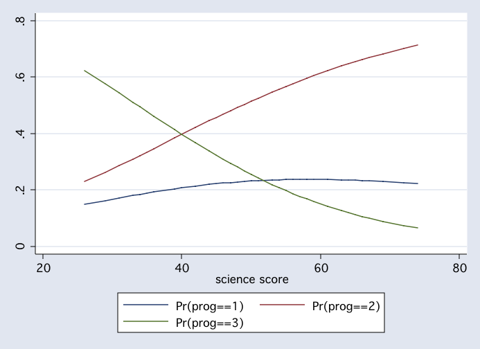
sort science
twoway connect p1 p2 p3 science, msym(i i i)
 summarize p1 p2 p3
Variable | Obs Mean Std. Dev. Min Max
-------------+--------------------------------------------------------
p1 | 200 .225 .0166541 .1483478 .2371181
p2 | 200 .525 .1044329 .2296548 .7127639
p3 | 200 .25 .119155 .0644656 .6219974
drop p1 p2 p3
summarize p1 p2 p3
Variable | Obs Mean Std. Dev. Min Max
-------------+--------------------------------------------------------
p1 | 200 .225 .0166541 .1483478 .2371181
p2 | 200 .525 .1044329 .2296548 .7127639
p3 | 200 .25 .119155 .0644656 .6219974
drop p1 p2 p3
Here are some more of the Long & Freeze utilities.
prchange

mlogit: Changes in Predicted Probabilities for prog

science
            Avg|Chg|     general    vocation    academic
Min->Max   .37168786   .07442269  -.55753179    .4831091
   -+1/2   .00786675   .00113033  -.01180014   .01066977
  -+sd/2   .07776304   .01132315  -.11664455   .10532141
MargEfct   .00786688   .00113019  -.01180032   .01067013

           general   vocation   academic
Pr(y|x)  .23351446  .23203561  .53444993

        science
    x=    51.85
sd(x)=  9.90089

prtab science


mlogit: Predicted probabilities for prog

Predicted probability of outcome 1 (general)

----------------------
science   |
score     | Prediction
----------+-----------
       26 |     0.1483
       29 |     0.1621
       31 |     0.1711
       33 |     0.1799
       34 |     0.1841
       35 |     0.1882
       36 |     0.1922
       39 |     0.2034
       40 |     0.2068
       42 |     0.2131
       44 |     0.2188
       45 |     0.2213
       46 |     0.2236
       47 |     0.2258
       48 |     0.2278
       49 |     0.2295
       50 |     0.2311
       51 |     0.2325
       53 |     0.2347
       54 |     0.2355
       55 |     0.2362
       56 |     0.2367
       57 |     0.2370
       58 |     0.2371
       59 |     0.2371
       61 |     0.2367
       63 |     0.2357
       64 |     0.2350
       65 |     0.2342
       66 |     0.2333
       67 |     0.2323
       69 |     0.2299
       72 |     0.2259
       74 |     0.2228
----------------------

Predicted probability of outcome 3 (vocation)

----------------------
science   |
score     | Prediction
----------+-----------
       26 |     0.6220
       29 |     0.5752
       31 |     0.5431
       33 |     0.5106
       34 |     0.4943
       35 |     0.4780
       36 |     0.4617
       39 |     0.4134
       40 |     0.3976
       42 |     0.3666
       44 |     0.3366
       45 |     0.3220
       46 |     0.3078
       47 |     0.2940
       48 |     0.2804
       49 |     0.2673
       50 |     0.2546
       51 |     0.2422
       53 |     0.2187
       54 |     0.2076
       55 |     0.1969
       56 |     0.1866
       57 |     0.1767
       58 |     0.1673
       59 |     0.1582
       61 |     0.1413
       63 |     0.1258
       64 |     0.1187
       65 |     0.1119
       66 |     0.1054
       67 |     0.0993
       69 |     0.0879
       72 |     0.0731
       74 |     0.0645
----------------------

Predicted probability of outcome 2 (academic)

----------------------
science   |
score     | Prediction
----------+-----------
       26 |     0.2297
       29 |     0.2627
       31 |     0.2857
       33 |     0.3095
       34 |     0.3216
       35 |     0.3338
       36 |     0.3461
       39 |     0.3832
       40 |     0.3956
       42 |     0.4203
       44 |     0.4446
       45 |     0.4567
       46 |     0.4685
       47 |     0.4802
       48 |     0.4918
       49 |     0.5032
       50 |     0.5143
       51 |     0.5253
       53 |     0.5466
       54 |     0.5569
       55 |     0.5669
       56 |     0.5767
       57 |     0.5863
       58 |     0.5956
       59 |     0.6047
       61 |     0.6221
       63 |     0.6385
       64 |     0.6463
       65 |     0.6539
       66 |     0.6613
       67 |     0.6685
       69 |     0.6821
       72 |     0.7011
       74 |     0.7128
----------------------

    science
x=    51.85

mlogtest, combine lrcomb

**** Wald tests for combining outcome categories

 Ho: All coefficients except intercepts associated with given pair
     of outcomes are 0 (i.e., categories can be collapsed).

Categories tested |      chi2   df   P>chi2
------------------+------------------------
 general-vocation |     6.449    1    0.011
 general-academic |     0.647    1    0.421
vocation-academic |    13.966    1    0.000
-------------------------------------------

**** LR tests for combining outcome categories

 Ho: All coefficients except intercepts associated with given pair
     of outcomes are 0 (i.e., categories can be collapsed).

Categories tested |      chi2   df   P>chi2
------------------+------------------------
 general-vocation |     6.776    1    0.009
 general-academic |     0.646    1    0.421
vocation-academic |    15.326    1    0.000
-------------------------------------------

tabstat science, by(prog)

Summary for variables: science
     by categories of: prog (type of program)

    prog |      mean
---------+----------
 general |  52.44444
academic |      53.8
vocation |     47.22
---------+----------
   Total |     51.85
A Two Predictor Example
mlogit prog science honors, nolog

Multinomial logistic regression                   Number of obs   =        200
                                                  LR chi2(4)      =      25.11
                                                  Prob > chi2     =     0.0000
Log likelihood = -191.54213                       Pseudo R2       =     0.0615

------------------------------------------------------------------------------
        prog |      Coef.   Std. Err.      z    P>|z|     [95% Conf. Interval]
-------------+----------------------------------------------------------------
general      |
     science |   .0065831   .0204231     0.32   0.747    -.0334454    .0466117
      honors |  -1.260566   .4881122    -2.58   0.010    -2.217248   -.3038836
       _cons |  -.8718198   1.060829    -0.82   0.411    -2.951007    1.207367
-------------+----------------------------------------------------------------
vocation     |
     science |  -.0530555   .0203973    -2.60   0.009    -.0930334   -.0130776
      honors |  -1.010628   .5178674    -1.95   0.051     -2.02563     .004373
       _cons |   2.171415   .9955349     2.18   0.029     .2202025    4.122628
------------------------------------------------------------------------------
(Outcome prog==academic is the comparison group)

test science

 ( 1)  [general]science = 0
 ( 2)  [vocation]science = 0

           chi2(  2) =    8.39
         Prob > chi2 =    0.0151

test honors

 ( 1)  [general]honors = 0
 ( 2)  [vocation]honors = 0

           chi2(  2) =    8.88
         Prob > chi2 =    0.0118

listcoef

mlogit (N=200): Factor Change in the Odds of prog

Variable: science (sd=     9.9)

    Odds comparing|
Group 1 vs Group 2|      b         z     P>|z|     e^b   e^bStdX
------------------+---------------------------------------------
general -vocation |   0.05964    2.537   0.011   1.0615   1.8048
general -academic |   0.00658    0.322   0.747   1.0066   1.0673
vocation-general  |  -0.05964   -2.537   0.011   0.9421   0.5541
vocation-academic |  -0.05306   -2.601   0.009   0.9483   0.5914
academic-general  |  -0.00658   -0.322   0.747   0.9934   0.9369
academic-vocation |   0.05306    2.601   0.009   1.0545   1.6910
----------------------------------------------------------------

Variable: honors (sd=     .44)

    Odds comparing|
Group 1 vs Group 2|      b         z     P>|z|     e^b   e^bStdX
------------------+---------------------------------------------
general -vocation |  -0.24994   -0.390   0.696   0.7788   0.8953
general -academic |  -1.26057   -2.583   0.010   0.2835   0.5725
vocation-general  |   0.24994    0.390   0.696   1.2839   1.1169
vocation-academic |  -1.01063   -1.952   0.051   0.3640   0.6395
academic-general  |   1.26057    2.583   0.010   3.5274   1.7467
academic-vocation |   1.01063    1.952   0.051   2.7473   1.5638
----------------------------------------------------------------

fitstat, using(M1)

Measures of Fit for mlogit of prog

                             Current            Saved       Difference
Model:                        mlogit           mlogit
N:                               200              200                0
Log-Lik Intercept Only:     -204.097         -204.097            0.000
Log-Lik Full Model:         -191.542         -196.024            4.482
D:                           383.084(194)     392.048(196)       8.964(2)
LR:                           25.109(4)        16.145(2)         8.964(2)
Prob > LR:                     0.000            0.000            0.011
McFadden's R2:                 0.062            0.040            0.022
McFadden's Adj R2:             0.032            0.020            0.012
Maximum Likelihood R2:         0.118            0.078            0.040
Cragg & Uhler's R2:            0.136            0.089            0.046
Count R2:                      0.540            0.525            0.015
Adj Count R2:                  0.032            0.000            0.032
AIC:                           1.975            2.000           -0.025
AIC*n:                       395.084          400.048           -4.964
BIC:                        -644.789         -646.422            1.633
BIC':                         -3.916           -5.548            1.633

Difference of    1.633 in BIC' provides weak support for saved model.

Note: p-value for difference in LR is only valid if models are nested.

mlogtest, combine lrcomb

**** Wald tests for combining outcome categories

 Ho: All coefficients except intercepts associated with given pair
     of outcomes are 0 (i.e., categories can be collapsed).

Categories tested |      chi2   df   P>chi2
------------------+------------------------
 general-vocation |     6.671    2    0.036
 general-academic |     7.042    2    0.030
vocation-academic |    16.139    2    0.000
-------------------------------------------

**** LR tests for combining outcome categories

 Ho: All coefficients except intercepts associated with given pair
     of outcomes are 0 (i.e., categories can be collapsed).

Categories tested |      chi2   df   P>chi2
------------------+------------------------
 general-vocation |     7.039    2    0.030
 general-academic |     8.175    2    0.017
vocation-academic |    19.387    2    0.000
-------------------------------------------

prtab science honors

mlogit: Predicted probabilities for prog

Predicted probability of outcome 1 (general)

--------------------------
science   |     honors
score     |      0       1
----------+---------------
       26 | 0.1340  0.0724
       29 | 0.1494  0.0785
       31 | 0.1600  0.0825
       33 | 0.1708  0.0866
       34 | 0.1763  0.0886
       35 | 0.1818  0.0906
       36 | 0.1874  0.0926
       39 | 0.2041  0.0985
       40 | 0.2097  0.1004
       42 | 0.2209  0.1042
       44 | 0.2320  0.1079
       45 | 0.2375  0.1097
       46 | 0.2429  0.1116
       47 | 0.2484  0.1133
       48 | 0.2537  0.1151
       49 | 0.2590  0.1168
       50 | 0.2643  0.1186
       51 | 0.2695  0.1203
       53 | 0.2796  0.1236
       54 | 0.2846  0.1252
       55 | 0.2895  0.1268
       56 | 0.2943  0.1284
       57 | 0.2991  0.1300
       58 | 0.3038  0.1315
       59 | 0.3083  0.1330
       61 | 0.3172  0.1360
       63 | 0.3258  0.1389
       64 | 0.3300  0.1403
       65 | 0.3341  0.1417
       66 | 0.3381  0.1431
       67 | 0.3420  0.1445
       69 | 0.3496  0.1472
       72 | 0.3604  0.1511
       74 | 0.3672  0.1536
--------------------------

Predicted probability of outcome 3 (vocation)

--------------------------
science   |     honors
score     |      0       1
----------+---------------
       26 | 0.5960  0.4133
       29 | 0.5556  0.3747
       31 | 0.5281  0.3499
       33 | 0.5005  0.3257
       34 | 0.4867  0.3140
       35 | 0.4729  0.3025
       36 | 0.4591  0.2913
       39 | 0.4183  0.2590
       40 | 0.4049  0.2488
       42 | 0.3785  0.2292
       44 | 0.3528  0.2107
       45 | 0.3402  0.2019
       46 | 0.3279  0.1933
       47 | 0.3158  0.1850
       48 | 0.3039  0.1770
       49 | 0.2923  0.1693
       50 | 0.2810  0.1619
       51 | 0.2699  0.1547
       53 | 0.2486  0.1411
       54 | 0.2384  0.1346
       55 | 0.2285  0.1285
       56 | 0.2188  0.1225
       57 | 0.2095  0.1169
       58 | 0.2004  0.1114
       59 | 0.1917  0.1062
       61 | 0.1750  0.0963
       63 | 0.1596  0.0873
       64 | 0.1522  0.0831
       65 | 0.1452  0.0791
       66 | 0.1384  0.0752
       67 | 0.1319  0.0716
       69 | 0.1197  0.0647
       72 | 0.1032  0.0555
       74 | 0.0933  0.0501
--------------------------

Predicted probability of outcome 2 (academic)

--------------------------
science   |     honors
score     |      0       1
----------+---------------
       26 | 0.2700  0.5143
       29 | 0.2951  0.5468
       31 | 0.3119  0.5676
       33 | 0.3287  0.5877
       34 | 0.3370  0.5974
       35 | 0.3453  0.6069
       36 | 0.3535  0.6161
       39 | 0.3776  0.6425
       40 | 0.3854  0.6508
       42 | 0.4006  0.6666
       44 | 0.4152  0.6814
       45 | 0.4223  0.6884
       46 | 0.4292  0.6951
       47 | 0.4358  0.7016
       48 | 0.4423  0.7079
       49 | 0.4486  0.7138
       50 | 0.4547  0.7196
       51 | 0.4606  0.7251
       53 | 0.4717  0.7354
       54 | 0.4770  0.7401
       55 | 0.4820  0.7447
       56 | 0.4868  0.7491
       57 | 0.4914  0.7532
       58 | 0.4958  0.7571
       59 | 0.5000  0.7608
       61 | 0.5077  0.7677
       63 | 0.5146  0.7738
       64 | 0.5178  0.7766
       65 | 0.5207  0.7792
       66 | 0.5235  0.7817
       67 | 0.5261  0.7840
       69 | 0.5307  0.7881
       72 | 0.5365  0.7934
       74 | 0.5395  0.7962
--------------------------

    science   honors
x=    51.85     .265
Categorical Predictor Example
tabulate ses, gen(ses)

        ses |      Freq.     Percent        Cum.
------------+-----------------------------------
        low |         47       23.50       23.50
     middle |         95       47.50       71.00
       high |         58       29.00      100.00
------------+-----------------------------------
      Total |        200      100.00

mlogit prog ses1 ses2, nolog

Multinomial logistic regression                   Number of obs   =        200
                                                  LR chi2(4)      =      16.78
                                                  Prob > chi2     =     0.0021
Log likelihood = -195.70519                       Pseudo R2       =     0.0411

------------------------------------------------------------------------------
        prog |      Coef.   Std. Err.      z    P>|z|     [95% Conf. Interval]
-------------+----------------------------------------------------------------
general      |
        ses1 |   1.368595   .5000526     2.74   0.006     .3885097     2.34868
        ses2 |   .7519877   .4556845     1.65   0.099    -.1411374    1.645113
       _cons |  -1.540445    .367316    -4.19   0.000    -2.260371   -.8205189
-------------+----------------------------------------------------------------
vocation     |
        ses1 |   1.332227   .5501167     2.42   0.015     .2540182    2.410436
        ses2 |   1.441557    .470796     3.06   0.002     .5188139      2.3643
       _cons |  -1.791759   .4082444    -4.39   0.000    -2.591904   -.9916151
------------------------------------------------------------------------------
(Outcome prog==academic is the comparison group)

test ses1 ses2

 ( 1)  [general]ses1 = 0
 ( 2)  [vocation]ses1 = 0
 ( 3)  [general]ses2 = 0
 ( 4)  [vocation]ses2 = 0

           chi2(  4) =   15.67
         Prob > chi2 =    0.0035
Final Model: Three Predictors
mlogit prog science honors ses1 ses2, nolog

Multinomial logistic regression                   Number of obs   =        200
                                                  LR chi2(8)      =      37.66
                                                  Prob > chi2     =     0.0000
Log likelihood = -185.26706                       Pseudo R2       =     0.0923

------------------------------------------------------------------------------
        prog |      Coef.   Std. Err.      z    P>|z|     [95% Conf. Interval]
-------------+----------------------------------------------------------------
general      |
     science |   .0196812   .0213451     0.92   0.357    -.0221545    .0615168
      honors |  -1.254872   .5053887    -2.48   0.013    -2.245416   -.2643289
        ses1 |   1.323819   .5279468     2.51   0.012     .2890618    2.358575
        ses2 |   .5173172   .4725885     1.09   0.274    -.4089392    1.443574
       _cons |  -2.146701   1.201467    -1.79   0.074    -4.501532    .2081308
-------------+----------------------------------------------------------------
vocation     |
     science |   -.052548   .0215222    -2.44   0.015    -.0947306   -.0103653
      honors |  -.8064186   .5309991    -1.52   0.129    -1.847158    .2343204
        ses1 |   .8638298   .5844485     1.48   0.139    -.2816682    2.009328
        ses2 |   1.167853   .4932099     2.37   0.018     .2011791    2.134526
       _cons |   1.280312   1.133052     1.13   0.258    -.9404289    3.501053
------------------------------------------------------------------------------
(Outcome prog==academic is the comparison group)

test science

 ( 1)  [general]science = 0
 ( 2)  [vocation]science = 0

           chi2(  2) =    9.28
         Prob > chi2 =    0.0097

test honors

 ( 1)  [general]honors = 0
 ( 2)  [vocation]honors = 0

           chi2(  2) =    7.25
         Prob > chi2 =    0.0267


test ses1 ses2

 ( 1)  [general]ses1 = 0
 ( 2)  [vocation]ses1 = 0
 ( 3)  [general]ses2 = 0
 ( 4)  [vocation]ses2 = 0

           chi2(  4) =    9.88
         Prob > chi2 =    0.0424

listcoef

mlogit (N=200): Factor Change in the Odds of prog

Variable: science (sd=     9.9)

    Odds comparing|
Group 1 vs Group 2|      b         z     P>|z|     e^b   e^bStdX
------------------+---------------------------------------------
general -vocation |   0.07223    2.905   0.004   1.0749   2.0445
general -academic |   0.01968    0.922   0.357   1.0199   1.2151
vocation-general  |  -0.07223   -2.905   0.004   0.9303   0.4891
vocation-academic |  -0.05255   -2.442   0.015   0.9488   0.5944
academic-general  |  -0.01968   -0.922   0.357   0.9805   0.8229
academic-vocation |   0.05255    2.442   0.015   1.0540   1.6825
----------------------------------------------------------------

Variable: honors (sd=     .44)

    Odds comparing|
Group 1 vs Group 2|      b         z     P>|z|     e^b   e^bStdX
------------------+---------------------------------------------
general -vocation |  -0.44845   -0.684   0.494   0.6386   0.8200
general -academic |  -1.25487   -2.483   0.013   0.2851   0.5740
vocation-general  |   0.44845    0.684   0.494   1.5659   1.2195
vocation-academic |  -0.80642   -1.519   0.129   0.4465   0.6999
academic-general  |   1.25487    2.483   0.013   3.5074   1.7423
academic-vocation |   0.80642    1.519   0.129   2.2399   1.4287
----------------------------------------------------------------

Variable: ses1 (sd=     .43)

    Odds comparing|
Group 1 vs Group 2|      b         z     P>|z|     e^b   e^bStdX
------------------+---------------------------------------------
general -vocation |   0.45999    0.688   0.491   1.5841   1.2159
general -academic |   1.32382    2.507   0.012   3.7577   1.7554
vocation-general  |  -0.45999   -0.688   0.491   0.6313   0.8224
vocation-academic |   0.86383    1.478   0.139   2.3722   1.4437
academic-general  |  -1.32382   -2.507   0.012   0.2661   0.5697
academic-vocation |  -0.86383   -1.478   0.139   0.4215   0.6927
----------------------------------------------------------------

Variable: ses2 (sd=      .5)

    Odds comparing|
Group 1 vs Group 2|      b         z     P>|z|     e^b   e^bStdX
------------------+---------------------------------------------
general -vocation |  -0.65054   -1.083   0.279   0.5218   0.7220
general -academic |   0.51732    1.095   0.274   1.6775   1.2956
vocation-general  |   0.65054    1.083   0.279   1.9166   1.3850
vocation-academic |   1.16785    2.368   0.018   3.2151   1.7944
academic-general  |  -0.51732   -1.095   0.274   0.5961   0.7718
academic-vocation |  -1.16785   -2.368   0.018   0.3110   0.5573
----------------------------------------------------------------

fitstat, using(M1)

Measures of Fit for mlogit of prog

                             Current            Saved       Difference
Model:                        mlogit           mlogit
N:                               200              200                0
Log-Lik Intercept Only:     -204.097         -204.097            0.000
Log-Lik Full Model:         -185.267         -196.024           10.757
D:                           370.534(190)     392.048(196)      21.514(6)
LR:                           37.659(8)        16.145(2)        21.514(6)
Prob > LR:                     0.000            0.000            0.001
McFadden's R2:                 0.092            0.040            0.053
McFadden's Adj R2:             0.043            0.020            0.023
Maximum Likelihood R2:         0.172            0.078            0.094
Cragg & Uhler's R2:            0.197            0.089            0.108
Count R2:                      0.575            0.525            0.050
Adj Count R2:                  0.105            0.000            0.105
AIC:                           1.953            2.000           -0.048
AIC*n:                       390.534          400.048           -9.514
BIC:                        -636.146         -646.422           10.276
BIC':                          4.727           -5.548           10.276

Difference of   10.276 in BIC' provides very strong support for saved model.

Note: p-value for difference in LR is only valid if models are nested.

prchange, x(honors=1 ses1=0 ses2=1)

mlogit: Changes in Predicted Probabilities for prog

science
            Avg|Chg|     general    vocation    academic
Min->Max   .31191427   .13955039  -.46787138   .32832104
   -+1/2    .0064501   .00306802  -.00967517   .00660712
  -+sd/2   .06380373   .03033344   -.0957056   .06537217
MargEfct   .00645018   .00306807  -.00967527    .0066072

honors
           Avg|Chg|    general   vocation   academic
    0->1  .15676552   -.132423  -.1027253  .23514825

ses1
            Avg|Chg|     general    vocation    academic
    0->1    .1669159   .14041305   .10996082  -.25037384

ses2
            Avg|Chg|     general    vocation    academic
    0->1   .11027237    .0266413   .13876726  -.16540855

           general   vocation   academic
Pr(y|x)  .10382493  .22670016   .6694749

        science   honors     ses1     ses2
    x=    51.85        1        0        1
sd(x)=  9.90089  .442441  .425063  .500628

prtab science honors, x(ses1=0 ses2=1)

mlogit: Predicted probabilities for prog

Predicted probability of outcome 1 (general)

--------------------------
science   |     honors
score     |      0       1
----------+---------------
       26 | 0.0765  0.0387
       29 | 0.0897  0.0445
       31 | 0.0994  0.0486
       33 | 0.1098  0.0530
       34 | 0.1153  0.0553
       35 | 0.1209  0.0576
       36 | 0.1267  0.0600
       39 | 0.1450  0.0674
       40 | 0.1514  0.0700
       42 | 0.1647  0.0753
       44 | 0.1784  0.0808
       45 | 0.1855  0.0836
       46 | 0.1927  0.0865
       47 | 0.1999  0.0893
       48 | 0.2073  0.0923
       49 | 0.2147  0.0952
       50 | 0.2222  0.0982
       51 | 0.2298  0.1012
       53 | 0.2451  0.1074
       54 | 0.2528  0.1105
       55 | 0.2605  0.1136
       56 | 0.2683  0.1168
       57 | 0.2761  0.1200
       58 | 0.2838  0.1233
       59 | 0.2916  0.1265
       61 | 0.3072  0.1331
       63 | 0.3226  0.1398
       64 | 0.3303  0.1432
       65 | 0.3380  0.1466
       66 | 0.3456  0.1500
       67 | 0.3532  0.1535
       69 | 0.3682  0.1604
       72 | 0.3903  0.1710
       74 | 0.4048  0.1782
--------------------------

Predicted probability of outcome 3 (vocation)

--------------------------
science   |     honors
score     |      0       1
----------+---------------
       26 | 0.6898  0.5465
       29 | 0.6517  0.5059
       31 | 0.6251  0.4787
       33 | 0.5976  0.4517
       34 | 0.5836  0.4382
       35 | 0.5694  0.4248
       36 | 0.5551  0.4116
       39 | 0.5116  0.3725
       40 | 0.4970  0.3598
       42 | 0.4678  0.3350
       44 | 0.4387  0.3111
       45 | 0.4242  0.2994
       46 | 0.4099  0.2880
       47 | 0.3957  0.2769
       48 | 0.3817  0.2660
       49 | 0.3678  0.2554
       50 | 0.3541  0.2451
       51 | 0.3407  0.2350
       53 | 0.3145  0.2158
       54 | 0.3018  0.2066
       55 | 0.2893  0.1976
       56 | 0.2772  0.1890
       57 | 0.2654  0.1807
       58 | 0.2538  0.1726
       59 | 0.2426  0.1648
       61 | 0.2212  0.1501
       63 | 0.2011  0.1364
       64 | 0.1915  0.1300
       65 | 0.1823  0.1238
       66 | 0.1734  0.1179
       67 | 0.1649  0.1122
       69 | 0.1488  0.1015
       72 | 0.1270  0.0871
       74 | 0.1140  0.0786
--------------------------

Predicted probability of outcome 2 (academic)

--------------------------
science   |     honors
score     |      0       1
----------+---------------
       26 | 0.2338  0.4149
       29 | 0.2586  0.4496
       31 | 0.2755  0.4727
       33 | 0.2926  0.4953
       34 | 0.3012  0.5065
       35 | 0.3097  0.5176
       36 | 0.3182  0.5284
       39 | 0.3434  0.5600
       40 | 0.3516  0.5701
       42 | 0.3675  0.5896
       44 | 0.3829  0.6081
       45 | 0.3903  0.6170
       46 | 0.3974  0.6255
       47 | 0.4044  0.6338
       48 | 0.4111  0.6417
       49 | 0.4175  0.6494
       50 | 0.4237  0.6567
       51 | 0.4295  0.6637
       53 | 0.4405  0.6769
       54 | 0.4455  0.6830
       55 | 0.4501  0.6887
       56 | 0.4545  0.6942
       57 | 0.4586  0.6993
       58 | 0.4623  0.7042
       59 | 0.4658  0.7087
       61 | 0.4716  0.7168
       63 | 0.4763  0.7238
       64 | 0.4781  0.7268
       65 | 0.4797  0.7296
       66 | 0.4810  0.7321
       67 | 0.4819  0.7344
       69 | 0.4830  0.7381
       72 | 0.4827  0.7418
       74 | 0.4812  0.7432
--------------------------

    science   honors     ses1     ses2
x=    51.85     .265        0        1