You can view movies of this seminar via the links below.
The purpose of this seminar is to give users an introduction to analyzing multinomial logistic models using Stata. In addition to the built-in Stata commands we will be demonstrating the use of a number on user-written ado’s, in particular, listcoef, fitstat, prchange, prtab, etc. To find out more about these programs or to download them type search followed by the program name in the Stata command window (example: search listcoef). These add-on programs ease the running and interpretation of ordinal logistic models.
Binary Response Variable Example
Let’s begin with an example using a binary response variable. We will see that the results of an multinomial logistic model are exactly the same as for a traditional logistic model.
use https://stats.idre.ucla.edu/stat/stata/seminars/stata_BeyondBinaryLogistic/honors, clear

logit honors female

Iteration 0:   log likelihood = -115.64441
Iteration 1:   log likelihood = -113.68907
Iteration 2:   log likelihood = -113.67691
Iteration 3:   log likelihood =  -113.6769

Logit estimates                                   Number of obs   =        200
                                                  LR chi2(1)      =       3.94
                                                  Prob > chi2     =     0.0473
Log likelihood =  -113.6769                       Pseudo R2       =     0.0170

------------------------------------------------------------------------------
      honors |      Coef.   Std. Err.      z    P>|z|     [95% Conf. Interval]
-------------+----------------------------------------------------------------
      female |   .6513707   .3336752     1.95   0.051    -.0026207    1.305362
       _cons |  -1.400088   .2631619    -5.32   0.000    -1.915876   -.8842998
------------------------------------------------------------------------------

mlogit honors female

Iteration 0:   log likelihood = -115.64441
Iteration 1:   log likelihood = -113.68907
Iteration 2:   log likelihood = -113.67691
Iteration 3:   log likelihood =  -113.6769

Multinomial logistic regression                   Number of obs   =        200
                                                  LR chi2(1)      =       3.94
                                                  Prob > chi2     =     0.0473
Log likelihood =  -113.6769                       Pseudo R2       =     0.0170

------------------------------------------------------------------------------
      honors |      Coef.   Std. Err.      z    P>|z|     [95% Conf. Interval]
-------------+----------------------------------------------------------------
1            |
      female |   .6513707   .3336752     1.95   0.051    -.0026207    1.305362
       _cons |  -1.400088   .2631619    -5.32   0.000    -1.915876   -.8842998
------------------------------------------------------------------------------
(Outcome honors==0 is the comparison group)

predict p0 p1
(option p assumed; predicted probabilities)

list female honors p0 p1 in 1/20, nolabel

     +---------------------------------------+
     | female   honors         p0         p1 |
     |---------------------------------------|
  1. |      1        0   .6788991   .3211009 |
  2. |      0        0   .8021978   .1978022 |
  3. |      0        0   .8021978   .1978022 |
  4. |      1        1   .6788991   .3211009 |
  5. |      1        1   .6788991   .3211009 |
     |---------------------------------------|
  6. |      0        0   .8021978   .1978022 |
  7. |      1        0   .6788991   .3211009 |
  8. |      1        0   .6788991   .3211009 |
  9. |      1        0   .6788991   .3211009 |
 10. |      1        0   .6788991   .3211009 |
     |---------------------------------------|
 11. |      1        1   .6788991   .3211009 |
 12. |      0        0   .8021978   .1978022 |
 13. |      0        0   .8021978   .1978022 |
 14. |      1        0   .6788991   .3211009 |
 15. |      1        0   .6788991   .3211009 |
     |---------------------------------------|
 16. |      1        0   .6788991   .3211009 |
 17. |      0        0   .8021978   .1978022 |
 18. |      1        0   .6788991   .3211009 |
 19. |      1        1   .6788991   .3211009 |
 20. |      1        0   .6788991   .3211009 |
     +---------------------------------------+
3-Category Response Variable Example
use https://stats.idre.ucla.edu/stat/stata/seminars/stata_BeyondBinaryLogistic/hsb2, clear
(highschool and beyond (200 cases))

codebook prog

prog                                                                                       type of program
----------------------------------------------------------------------------------------------------------

                  type:  numeric (float)
                 label:  sel

                 range:  [1,3]                        units:  1
         unique values:  3                        missing .:  0/200

            tabulation:  Freq.   Numeric  Label
                            45         1  general
                           105         2  academic
                            50         3  vocation

mlogit prog female

Iteration 0:   log likelihood = -204.09667
Iteration 1:   log likelihood = -204.07028
Iteration 2:   log likelihood = -204.07028

Multinomial logistic regression                   Number of obs   =        200
                                                  LR chi2(2)      =       0.05
                                                  Prob > chi2     =     0.9739
Log likelihood = -204.07028                       Pseudo R2       =     0.0001

------------------------------------------------------------------------------
        prog |      Coef.   Std. Err.      z    P>|z|     [95% Conf. Interval]
-------------+----------------------------------------------------------------
general      |
      female |   -.076764   .3574964    -0.21   0.830    -.7774441    .6239161
       _cons |  -.8056252   .2624798    -3.07   0.002    -1.320076   -.2911742
-------------+----------------------------------------------------------------
vocation     |
      female |  -.0499528    .345012    -0.14   0.885    -.7261638    .6262583
       _cons |  -.7146534   .2544698    -2.81   0.005    -1.213405   -.2159018
------------------------------------------------------------------------------
(Outcome prog==academic is the comparison group)

mlogit, rrr                                /*  relative risk ratios  */

Multinomial logistic regression                   Number of obs   =        200
                                                  LR chi2(2)      =       0.05
                                                  Prob > chi2     =     0.9739
Log likelihood = -204.07028                       Pseudo R2       =     0.0001

------------------------------------------------------------------------------
        prog |        RRR   Std. Err.      z    P>|z|     [95% Conf. Interval]
-------------+----------------------------------------------------------------
general      |
      female |   .9261084   .3310804    -0.21   0.830     .4595791    1.866222
-------------+----------------------------------------------------------------
vocation     |
      female |   .9512744   .3282011    -0.14   0.885     .4837612    1.870598
------------------------------------------------------------------------------
(Outcome prog==academic is the comparison group)
Next, we look at some of the Long & Freese utilities.
listcoef

mlogit (N=200): Factor Change in the Odds of prog

Variable: female (sd=      .5)

    Odds comparing|
Group 1 vs Group 2|      b         z     P>|z|     e^b   e^bStdX
------------------+---------------------------------------------
general -vocation |  -0.02681   -0.065   0.948   0.9735   0.9867
general -academic |  -0.07676   -0.215   0.830   0.9261   0.9624
vocation-general  |   0.02681    0.065   0.948   1.0272   1.0135
vocation-academic |  -0.04995   -0.145   0.885   0.9513   0.9754
academic-general  |   0.07676    0.215   0.830   1.0798   1.0391
academic-vocation |   0.04995    0.145   0.885   1.0512   1.0253
----------------------------------------------------------------

listcoef, percent

mlogit (N=200): Percentage Change in the Odds of prog

Variable: female (sd=      .5)

    Odds comparing|
Group 1 vs Group 2|      b         z     P>|z|       %     %StdX
------------------+---------------------------------------------
general -vocation |  -0.02681   -0.065   0.948     -2.6     -1.3
general -academic |  -0.07676   -0.215   0.830     -7.4     -3.8
vocation-general  |   0.02681    0.065   0.948      2.7      1.3
vocation-academic |  -0.04995   -0.145   0.885     -4.9     -2.5
academic-general  |   0.07676    0.215   0.830      8.0      3.9
academic-vocation |   0.04995    0.145   0.885      5.1      2.5
----------------------------------------------------------------

fitstat

Measures of Fit for mlogit of prog

Log-Lik Intercept Only:     -204.097     Log-Lik Full Model:         -204.070
D(196):                      408.141     LR(2):                         0.053
                                         Prob > LR:                     0.974
McFadden's R2:                 0.000     McFadden's Adj R2:            -0.019
Maximum Likelihood R2:         0.000     Cragg & Uhler's R2:            0.000
Count R2:                      0.525     Adj Count R2:                  0.000
AIC:                           2.081     AIC*n:                       416.141
BIC:                        -630.330     BIC':                         10.544

prchange

mlogit: Changes in Predicted Probabilities for prog

female
            Avg|Chg|     general    vocation    academic
    0->1   .01041771  -.01058574  -.00504084   .01562655

           general   vocation   academic
Pr(y|x)  .22496811  .25002041  .52501148

        female
    x=    .545
sd(x)=  .49922

prtab female

mlogit: Predicted probabilities for prog

Predicted probability of outcome 1 (general)

----------------------
   female | Prediction
----------+-----------
     male |     0.2308
   female |     0.2202
----------------------

Predicted probability of outcome 3 (vocation)

----------------------
   female | Prediction
----------+-----------
     male |     0.2527
   female |     0.2477
----------------------

Predicted probability of outcome 2 (academic)

----------------------
   female | Prediction
----------+-----------
     male |     0.5165
   female |     0.5321
----------------------

    female
x=    .545

predict p1 p2 p3
(option p assumed; predicted probabilities)

list female prog p1 p2 p3 in 1/20, nolabel

     +------------------------------------------------+
     | female   prog         p1         p2         p3 |
     |------------------------------------------------|
  1. |      0      1   .2307692   .5164835   .2527473 |
  2. |      1      3   .2201835   .5321101   .2477064 |
  3. |      0      1   .2307692   .5164835   .2527473 |
  4. |      0      3   .2307692   .5164835   .2527473 |
  5. |      0      2   .2307692   .5164835   .2527473 |
     |------------------------------------------------|
  6. |      0      2   .2307692   .5164835   .2527473 |
  7. |      0      1   .2307692   .5164835   .2527473 |
  8. |      0      2   .2307692   .5164835   .2527473 |
  9. |      0      1   .2307692   .5164835   .2527473 |
 10. |      0      2   .2307692   .5164835   .2527473 |
     |------------------------------------------------|
 11. |      0      3   .2307692   .5164835   .2527473 |
 12. |      0      2   .2307692   .5164835   .2527473 |
 13. |      0      2   .2307692   .5164835   .2527473 |
 14. |      0      2   .2307692   .5164835   .2527473 |
 15. |      0      2   .2307692   .5164835   .2527473 |
     |------------------------------------------------|
 16. |      0      1   .2307692   .5164835   .2527473 |
 17. |      0      2   .2307692   .5164835   .2527473 |
 18. |      0      1   .2307692   .5164835   .2527473 |
 19. |      0      2   .2307692   .5164835   .2527473 |
 20. |      0      1   .2307692   .5164835   .2527473 |
     +------------------------------------------------+

drop p1 p2 p3
An Example Using a Continuous Predictor
mlogit prog read
Iteration 0: log likelihood = -204.09667
Iteration 1: log likelihood = -185.28771
Iteration 2: log likelihood = -184.59416
Iteration 3: log likelihood = -184.58662
Iteration 4: log likelihood = -184.58661
Multinomial logistic regression Number of obs = 200
LR chi2(2) = 39.02
Prob > chi2 = 0.0000
Log likelihood = -184.58661 Pseudo R2 = 0.0956
------------------------------------------------------------------------------
prog | Coef. Std. Err. z P>|z| [95% Conf. Interval]
-------------+----------------------------------------------------------------
general |
read | -.0703559 .0200906 -3.50 0.000 -.1097328 -.0309791
_cons | 2.874114 1.054187 2.73 0.006 .8079463 4.940282
-------------+----------------------------------------------------------------
vocation |
read | -.1164723 .0223442 -5.21 0.000 -.1602662 -.0726784
_cons | 5.189645 1.116495 4.65 0.000 3.001355 7.377934
------------------------------------------------------------------------------
(Outcome prog==academic is the comparison group)
listcoef
mlogit (N=200): Factor Change in the Odds of prog
Variable: read (sd= 10)
Odds comparing|
Group 1 vs Group 2| b z P>|z| e^b e^bStdX
------------------+---------------------------------------------
general -vocation | 0.04612 1.924 0.054 1.0472 1.6045
general -academic | -0.07036 -3.502 0.000 0.9321 0.4861
vocation-general | -0.04612 -1.924 0.054 0.9549 0.6232
vocation-academic | -0.11647 -5.213 0.000 0.8901 0.3030
academic-general | 0.07036 3.502 0.000 1.0729 2.0572
academic-vocation | 0.11647 5.213 0.000 1.1235 3.3009
----------------------------------------------------------------
fitstat
Measures of Fit for mlogit of prog
Log-Lik Intercept Only: -204.097 Log-Lik Full Model: -184.587
D(196): 369.173 LR(2): 39.020
Prob > LR: 0.000
McFadden's R2: 0.096 McFadden's Adj R2: 0.076
Maximum Likelihood R2: 0.177 Cragg & Uhler's R2: 0.204
Count R2: 0.585 Adj Count R2: 0.126
AIC: 1.886 AIC*n: 377.173
BIC: -669.297 BIC': -28.423
predict p1 p2 p3
(option p assumed; predicted probabilities)
list read prog p1 p2 p3 in 1/20, nolabel
+----------------------------------------------+
| read prog p1 p2 p3 |
|----------------------------------------------|
1. | 57 1 .2063555 .6427623 .1508822 |
2. | 68 3 .1220411 .8242286 .0537303 |
3. | 44 1 .2793571 .3486395 .3720033 |
4. | 63 3 .1585986 .7534682 .0879332 |
5. | 47 2 .2702068 .4164652 .3133279 |
|----------------------------------------------|
6. | 44 2 .2793571 .3486395 .3720033 |
7. | 50 1 .2555427 .4864202 .2580371 |
8. | 34 2 .2681388 .1655863 .5662749 |
9. | 63 1 .1585986 .7534682 .0879332 |
10. | 57 2 .2063555 .6427623 .1508822 |
|----------------------------------------------|
11. | 60 3 .182365 .7015224 .1161126 |
12. | 57 2 .2063555 .6427623 .1508822 |
13. | 73 2 .091319 .8767558 .0319252 |
14. | 54 2 .229263 .5782328 .1925042 |
15. | 45 2 .2769624 .3708454 .3521922 |
|----------------------------------------------|
16. | 42 1 .2821275 .3058806 .4119919 |
17. | 47 2 .2702068 .4164652 .3133279 |
18. | 57 1 .2063555 .6427623 .1508822 |
19. | 68 2 .1220411 .8242286 .0537303 |
20. | 55 1 .2218377 .6002877 .1778745 |
+----------------------------------------------+
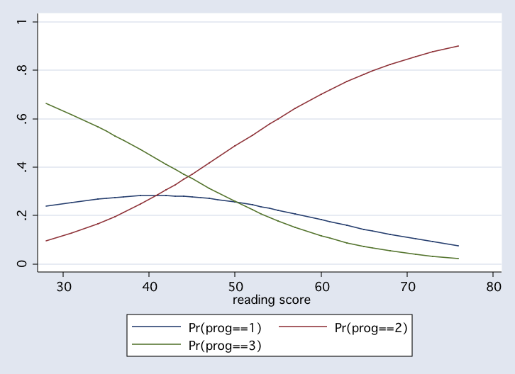
sort read
scatter p1 p2 p3 read, connect(l l l) msym(i i i)
 summarize p1 p2 p3
Variable | Obs Mean Std. Dev. Min Max
-------------+--------------------------------------------------------
p1 | 200 .225 .0582549 .0759783 .2825051
p2 | 200 .525 .2033302 .0966327 .9008916
p3 | 200 .25 .1509281 .0231301 .6647014
list read p1 p2 p3 if p1>p2
+---------------------------------------+
| read p1 p2 p3 |
|---------------------------------------|
1. | 28 .2386659 .0966327 .6647014 |
2. | 31 .2547603 .1273887 .617851 |
3. | 34 .2681388 .1655863 .5662749 |
4. | 34 .2681388 .1655863 .5662749 |
5. | 34 .2681388 .1655863 .5662749 |
|---------------------------------------|
6. | 34 .2681388 .1655863 .5662749 |
7. | 34 .2681388 .1655863 .5662749 |
8. | 34 .2681388 .1655863 .5662749 |
9. | 35 .2717949 .1800783 .5481268 |
10. | 36 .2749785 .1954673 .5295542 |
|---------------------------------------|
11. | 36 .2749785 .1954673 .5295542 |
12. | 36 .2749785 .1954673 .5295542 |
13. | 37 .2776492 .2117517 .5105991 |
14. | 37 .2776492 .2117517 .5105991 |
15. | 39 .2813043 .2469546 .4717411 |
|---------------------------------------|
16. | 39 .2813043 .2469546 .4717411 |
17. | 39 .2813043 .2469546 .4717411 |
18. | 39 .2813043 .2469546 .4717411 |
19. | 39 .2813043 .2469546 .4717411 |
20. | 39 .2813043 .2469546 .4717411 |
|---------------------------------------|
21. | 39 .2813043 .2469546 .4717411 |
22. | 39 .2813043 .2469546 .4717411 |
+---------------------------------------+
list read prog p1 p2 p3 if p1>p2 & p1>p3
drop p1 p2 p3
summarize p1 p2 p3
Variable | Obs Mean Std. Dev. Min Max
-------------+--------------------------------------------------------
p1 | 200 .225 .0582549 .0759783 .2825051
p2 | 200 .525 .2033302 .0966327 .9008916
p3 | 200 .25 .1509281 .0231301 .6647014
list read p1 p2 p3 if p1>p2
+---------------------------------------+
| read p1 p2 p3 |
|---------------------------------------|
1. | 28 .2386659 .0966327 .6647014 |
2. | 31 .2547603 .1273887 .617851 |
3. | 34 .2681388 .1655863 .5662749 |
4. | 34 .2681388 .1655863 .5662749 |
5. | 34 .2681388 .1655863 .5662749 |
|---------------------------------------|
6. | 34 .2681388 .1655863 .5662749 |
7. | 34 .2681388 .1655863 .5662749 |
8. | 34 .2681388 .1655863 .5662749 |
9. | 35 .2717949 .1800783 .5481268 |
10. | 36 .2749785 .1954673 .5295542 |
|---------------------------------------|
11. | 36 .2749785 .1954673 .5295542 |
12. | 36 .2749785 .1954673 .5295542 |
13. | 37 .2776492 .2117517 .5105991 |
14. | 37 .2776492 .2117517 .5105991 |
15. | 39 .2813043 .2469546 .4717411 |
|---------------------------------------|
16. | 39 .2813043 .2469546 .4717411 |
17. | 39 .2813043 .2469546 .4717411 |
18. | 39 .2813043 .2469546 .4717411 |
19. | 39 .2813043 .2469546 .4717411 |
20. | 39 .2813043 .2469546 .4717411 |
|---------------------------------------|
21. | 39 .2813043 .2469546 .4717411 |
22. | 39 .2813043 .2469546 .4717411 |
+---------------------------------------+
list read prog p1 p2 p3 if p1>p2 & p1>p3
drop p1 p2 p3
Here are some more of the Long & Freeze utilities.
prchange

mlogit: Changes in Predicted Probabilities for prog

read
            Avg|Chg|     general    vocation    academic
Min->Max   .53617262  -.16268767  -.64157127   .80425891
   -+1/2   .01529801  -.00669396  -.01625305   .02294701
  -+sd/2   .15414272  -.06625439   -.1649597   .23121408
MargEfct    .0153006  -.00669624  -.01625465   .02295089

           general   vocation   academic
Pr(y|x)  .24166824  .22017884  .53815293

           read
    x=    52.23
sd(x)=  10.2529

prtab read

mlogit: Predicted probabilities for prog

Predicted probability of outcome 1 (general)

----------------------
reading   |
score     | Prediction
----------+-----------
       28 |     0.2387
       31 |     0.2548
       34 |     0.2681
       35 |     0.2718
       36 |     0.2750
       37 |     0.2776
       39 |     0.2813
       41 |     0.2825
       42 |     0.2821
       43 |     0.2811
       44 |     0.2794
       45 |     0.2770
       46 |     0.2739
       47 |     0.2702
       48 |     0.2659
       50 |     0.2555
       52 |     0.2432
       53 |     0.2364
       54 |     0.2293
       55 |     0.2218
       57 |     0.2064
       60 |     0.1824
       61 |     0.1744
       63 |     0.1586
       65 |     0.1434
       66 |     0.1361
       68 |     0.1220
       71 |     0.1028
       73 |     0.0913
       76 |     0.0760
----------------------

Predicted probability of outcome 3 (vocation)

----------------------
reading   |
score     | Prediction
----------+-----------
       28 |     0.6647
       31 |     0.6179
       34 |     0.5663
       35 |     0.5481
       36 |     0.5296
       37 |     0.5106
       39 |     0.4717
       41 |     0.4320
       42 |     0.4120
       43 |     0.3920
       44 |     0.3720
       45 |     0.3522
       46 |     0.3326
       47 |     0.3133
       48 |     0.2944
       50 |     0.2580
       52 |     0.2239
       53 |     0.2079
       54 |     0.1925
       55 |     0.1779
       57 |     0.1509
       60 |     0.1161
       61 |     0.1060
       63 |     0.0879
       65 |     0.0725
       66 |     0.0657
       68 |     0.0537
       71 |     0.0394
       73 |     0.0319
       76 |     0.0231
----------------------

Predicted probability of outcome 2 (academic)

----------------------
reading   |
score     | Prediction
----------+-----------
       28 |     0.0966
       31 |     0.1274
       34 |     0.1656
       35 |     0.1801
       36 |     0.1955
       37 |     0.2118
       39 |     0.2470
       41 |     0.2855
       42 |     0.3059
       43 |     0.3270
       44 |     0.3486
       45 |     0.3708
       46 |     0.3935
       47 |     0.4165
       48 |     0.4397
       50 |     0.4864
       52 |     0.5329
       53 |     0.5557
       54 |     0.5782
       55 |     0.6003
       57 |     0.6428
       60 |     0.7015
       61 |     0.7196
       63 |     0.7535
       65 |     0.7841
       66 |     0.7983
       68 |     0.8242
       71 |     0.8577
       73 |     0.8768
       76 |     0.9009
----------------------

     read
x=  52.23

mlogtest, combine lrcomb

**** Wald tests for combining outcome categories

 Ho: All coefficients except intercepts associated with given pair
     of outcomes are 0 (i.e., categories can be collapsed).

Categories tested |      chi2   df   P>chi2
------------------+------------------------
 general-vocation |     3.703    1    0.054
 general-academic |    12.264    1    0.000
vocation-academic |    27.172    1    0.000
-------------------------------------------

**** LR tests for combining outcome categories

 Ho: All coefficients except intercepts associated with given pair
     of outcomes are 0 (i.e., categories can be collapsed).

Categories tested |      chi2   df   P>chi2
------------------+------------------------
 general-vocation |     3.838    1    0.050
 general-academic |    13.660    1    0.000
vocation-academic |    35.553    1    0.000
-------------------------------------------
A Two Predictor Example
mlogit prog read female

Iteration 0:   log likelihood = -204.09667
Iteration 1:   log likelihood = -185.12283
Iteration 2:   log likelihood = -184.41244
Iteration 3:   log likelihood = -184.40469
Iteration 4:   log likelihood = -184.40469

Multinomial logistic regression                   Number of obs   =        200
                                                  LR chi2(4)      =      39.38
                                                  Prob > chi2     =     0.0000
Log likelihood = -184.40469                       Pseudo R2       =     0.0965

------------------------------------------------------------------------------
        prog |      Coef.   Std. Err.      z    P>|z|     [95% Conf. Interval]
-------------+----------------------------------------------------------------
general      |
        read |  -.0712123   .0202062    -3.52   0.000    -.1108158   -.0316089
      female |  -.1834744   .3726879    -0.49   0.623    -.9139293    .5469805
       _cons |   3.019251   1.096285     2.75   0.006     .8705724     5.16793
-------------+----------------------------------------------------------------
vocation     |
        read |  -.1172833   .0224395    -5.23   0.000     -.161264   -.0733026
      female |   -.193847   .3800557    -0.51   0.610    -.9387425    .5510486
       _cons |    5.33822   1.156404     4.62   0.000      3.07171     7.60473
------------------------------------------------------------------------------
(Outcome prog==academic is the comparison group)

listcoef

mlogit (N=200): Factor Change in the Odds of prog

Variable: read (sd=      10)

    Odds comparing|
Group 1 vs Group 2|      b         z     P>|z|     e^b   e^bStdX
------------------+---------------------------------------------
general -vocation |   0.04607    1.922   0.055   1.0471   1.6038
general -academic |  -0.07121   -3.524   0.000   0.9313   0.4818
vocation-general  |  -0.04607   -1.922   0.055   0.9550   0.6235
vocation-academic |  -0.11728   -5.227   0.000   0.8893   0.3004
academic-general  |   0.07121    3.524   0.000   1.0738   2.0754
academic-vocation |   0.11728    5.227   0.000   1.1244   3.3284
----------------------------------------------------------------

Variable: female (sd=      .5)

    Odds comparing|
Group 1 vs Group 2|      b         z     P>|z|     e^b   e^bStdX
------------------+---------------------------------------------
general -vocation |   0.01037    0.025   0.980   1.0104   1.0052
general -academic |  -0.18347   -0.492   0.623   0.8324   0.9125
vocation-general  |  -0.01037   -0.025   0.980   0.9897   0.9948
vocation-academic |  -0.19385   -0.510   0.610   0.8238   0.9078
academic-general  |   0.18347    0.492   0.623   1.2014   1.0959
academic-vocation |   0.19385    0.510   0.610   1.2139   1.1016
----------------------------------------------------------------

fitstat

Measures of Fit for mlogit of prog

Log-Lik Intercept Only:     -204.097     Log-Lik Full Model:         -184.405
D(194):                      368.809     LR(4):                        39.384
                                         Prob > LR:                     0.000
McFadden's R2:                 0.096     McFadden's Adj R2:             0.067
Maximum Likelihood R2:         0.179     Cragg & Uhler's R2:            0.205
Count R2:                      0.590     Adj Count R2:                  0.137
AIC:                           1.904     AIC*n:                       380.809
BIC:                        -659.064     BIC':                        -18.191

mlogtest, combine lrcomb

**** Wald tests for combining outcome categories

 Ho: All coefficients except intercepts associated with given pair
     of outcomes are 0 (i.e., categories can be collapsed).

Categories tested |      chi2   df   P>chi2
------------------+------------------------
 general-vocation |     3.697    2    0.157
 general-academic |    12.455    2    0.002
vocation-academic |    27.333    2    0.000
-------------------------------------------

**** LR tests for combining outcome categories

 Ho: All coefficients except intercepts associated with given pair
     of outcomes are 0 (i.e., categories can be collapsed).

Categories tested |      chi2   df   P>chi2
------------------+------------------------
 general-vocation |     3.833    2    0.147
 general-academic |    13.916    2    0.001
vocation-academic |    35.841    2    0.000
-------------------------------------------

prtab read female

mlogit: Predicted probabilities for prog

Predicted probability of outcome 1 (general)

--------------------------
reading   |     female
score     |   male  female
----------+---------------
       28 | 0.2406  0.2381
       31 | 0.2577  0.2535
       34 | 0.2723  0.2659
       35 | 0.2764  0.2692
       36 | 0.2801  0.2719
       37 | 0.2833  0.2742
       39 | 0.2881  0.2769
       41 | 0.2905  0.2771
       42 | 0.2907  0.2762
       43 | 0.2902  0.2746
       44 | 0.2890  0.2724
       45 | 0.2872  0.2694
       46 | 0.2846  0.2659
       47 | 0.2814  0.2617
       48 | 0.2775  0.2569
       50 | 0.2678  0.2457
       52 | 0.2559  0.2327
       53 | 0.2492  0.2257
       54 | 0.2422  0.2183
       55 | 0.2347  0.2107
       57 | 0.2191  0.1951
       60 | 0.1944  0.1712
       61 | 0.1861  0.1633
       63 | 0.1696  0.1479
       65 | 0.1536  0.1331
       66 | 0.1459  0.1261
       68 | 0.1310  0.1127
       71 | 0.1105  0.0944
       73 | 0.0981  0.0836
       76 | 0.0816  0.0692
--------------------------

Predicted probability of outcome 3 (vocation)

--------------------------
reading   |     female
score     |   male  female
----------+---------------
       28 | 0.6731  0.6593
       31 | 0.6279  0.6113
       34 | 0.5780  0.5585
       35 | 0.5603  0.5399
       36 | 0.5422  0.5209
       37 | 0.5237  0.5016
       39 | 0.4857  0.4619
       41 | 0.4466  0.4216
       42 | 0.4268  0.4013
       43 | 0.4069  0.3810
       44 | 0.3870  0.3609
       45 | 0.3672  0.3410
       46 | 0.3475  0.3213
       47 | 0.3281  0.3020
       48 | 0.3090  0.2831
       50 | 0.2720  0.2470
       52 | 0.2370  0.2133
       53 | 0.2204  0.1975
       54 | 0.2045  0.1825
       55 | 0.1893  0.1682
       57 | 0.1612  0.1420
       60 | 0.1246  0.1085
       61 | 0.1139  0.0989
       63 | 0.0947  0.0817
       65 | 0.0782  0.0670
       66 | 0.0709  0.0606
       68 | 0.0580  0.0494
       71 | 0.0426  0.0361
       73 | 0.0345  0.0291
       76 | 0.0250  0.0210
--------------------------

Predicted probability of outcome 2 (academic)

--------------------------
reading   |     female
score     |   male  female
----------+---------------
       28 | 0.0863  0.1026
       31 | 0.1144  0.1352
       34 | 0.1497  0.1756
       35 | 0.1632  0.1909
       36 | 0.1776  0.2071
       37 | 0.1929  0.2243
       39 | 0.2262  0.2612
       41 | 0.2630  0.3013
       42 | 0.2826  0.3225
       43 | 0.3029  0.3444
       44 | 0.3240  0.3667
       45 | 0.3456  0.3896
       46 | 0.3678  0.4128
       47 | 0.3905  0.4363
       48 | 0.4135  0.4600
       50 | 0.4602  0.5073
       52 | 0.5071  0.5540
       53 | 0.5303  0.5768
       54 | 0.5533  0.5992
       55 | 0.5759  0.6211
       57 | 0.6198  0.6629
       60 | 0.6810  0.7203
       61 | 0.7000  0.7378
       63 | 0.7357  0.7705
       65 | 0.7682  0.7998
       66 | 0.7833  0.8133
       68 | 0.8110  0.8379
       71 | 0.8469  0.8695
       73 | 0.8673  0.8873
       76 | 0.8934  0.9098
--------------------------

      read  female
x=   52.23    .545
Categorical Predictor Example
tabulate ses, gen(ses)

        ses |      Freq.     Percent        Cum.
------------+-----------------------------------
        low |         47       23.50       23.50
     middle |         95       47.50       71.00
       high |         58       29.00      100.00
------------+-----------------------------------
      Total |        200      100.00

mlogit prog ses1 ses2

Iteration 0:   log likelihood = -204.09667
Iteration 1:   log likelihood = -195.82855
Iteration 2:   log likelihood = -195.70541
Iteration 3:   log likelihood = -195.70519

Multinomial logistic regression                   Number of obs   =        200
                                                  LR chi2(4)      =      16.78
                                                  Prob > chi2     =     0.0021
Log likelihood = -195.70519                       Pseudo R2       =     0.0411

------------------------------------------------------------------------------
        prog |      Coef.   Std. Err.      z    P>|z|     [95% Conf. Interval]
-------------+----------------------------------------------------------------
general      |
        ses1 |   1.368595   .5000526     2.74   0.006     .3885097     2.34868
        ses2 |   .7519877   .4556845     1.65   0.099    -.1411374    1.645113
       _cons |  -1.540445    .367316    -4.19   0.000    -2.260371   -.8205189
-------------+----------------------------------------------------------------
vocation     |
        ses1 |   1.332227   .5501167     2.42   0.015     .2540182    2.410436
        ses2 |   1.441557    .470796     3.06   0.002     .5188139      2.3643
       _cons |  -1.791759   .4082444    -4.39   0.000    -2.591904   -.9916151
------------------------------------------------------------------------------
(Outcome prog==academic is the comparison group)

test ses1 ses2

 ( 1)  [general]ses1 = 0
 ( 2)  [vocation]ses1 = 0
 ( 3)  [general]ses2 = 0
 ( 4)  [vocation]ses2 = 0

           chi2(  4) =   15.67
         Prob > chi2 =    0.0035
Final Model: Three Predictors
mlogit prog read female ses1 ses2

Iteration 0:   log likelihood = -204.09667
Iteration 1:   log likelihood = -180.65991
Iteration 2:   log likelihood = -179.41794
Iteration 3:   log likelihood = -179.38722
Iteration 4:   log likelihood = -179.38719

Multinomial logistic regression                   Number of obs   =        200
                                                  LR chi2(8)      =      49.42
                                                  Prob > chi2     =     0.0000
Log likelihood = -179.38719                       Pseudo R2       =     0.1211

------------------------------------------------------------------------------
        prog |      Coef.   Std. Err.      z    P>|z|     [95% Conf. Interval]
-------------+----------------------------------------------------------------
general      |
        read |  -.0622009    .020823    -2.99   0.003    -.1030132   -.0213887
      female |  -.2907466   .3827223    -0.76   0.447    -1.040869    .4593754
        ses1 |   1.053428   .5290998     1.99   0.046     .0164118    2.090445
        ses2 |   .5927571   .4697164     1.26   0.207    -.3278702    1.513384
       _cons |   2.057293   1.205372     1.71   0.088    -.3051927    4.419779
-------------+----------------------------------------------------------------
vocation     |
        read |  -.1153246   .0235584    -4.90   0.000    -.1614982    -.069151
      female |  -.2128803   .3916879    -0.54   0.587    -.9805745    .5548139
        ses1 |   .7672021   .6016694     1.28   0.202    -.4120482    1.946452
        ses2 |   1.222412     .50843     2.40   0.016     .2259076    2.218917
       _cons |   4.415091   1.272291     3.47   0.001     1.921447    6.908735
------------------------------------------------------------------------------
(Outcome prog==academic is the comparison group)

test ses1 ses2

 ( 1)  [general]ses1 = 0
 ( 2)  [vocation]ses1 = 0
 ( 3)  [general]ses2 = 0
 ( 4)  [vocation]ses2 = 0

           chi2(  4) =    9.88
         Prob > chi2 =    0.0424

listcoef

mlogit (N=200): Factor Change in the Odds of prog

Variable: read (sd=      10)

    Odds comparing|
Group 1 vs Group 2|      b         z     P>|z|     e^b   e^bStdX
------------------+---------------------------------------------
general -vocation |   0.05312    2.117   0.034   1.0546   1.7240
general -academic |  -0.06220   -2.987   0.003   0.9397   0.5285
vocation-general  |  -0.05312   -2.117   0.034   0.9483   0.5800
vocation-academic |  -0.11532   -4.895   0.000   0.8911   0.3065
academic-general  |   0.06220    2.987   0.003   1.0642   1.8922
academic-vocation |   0.11532    4.895   0.000   1.1222   3.2622
----------------------------------------------------------------

Variable: female (sd=      .5)

    Odds comparing|
Group 1 vs Group 2|      b         z     P>|z|     e^b   e^bStdX
------------------+---------------------------------------------
general -vocation |  -0.07787   -0.181   0.856   0.9251   0.9619
general -academic |  -0.29075   -0.760   0.447   0.7477   0.8649
vocation-general  |   0.07787    0.181   0.856   1.0810   1.0396
vocation-academic |  -0.21288   -0.543   0.587   0.8083   0.8992
academic-general  |   0.29075    0.760   0.447   1.3374   1.1562
academic-vocation |   0.21288    0.543   0.587   1.2372   1.1121
----------------------------------------------------------------

Variable: ses1 (sd=     .43)

    Odds comparing|
Group 1 vs Group 2|      b         z     P>|z|     e^b   e^bStdX
------------------+---------------------------------------------
general -vocation |   0.28623    0.435   0.663   1.3314   1.1294
general -academic |   1.05343    1.991   0.046   2.8675   1.5648
vocation-general  |  -0.28623   -0.435   0.663   0.7511   0.8854
vocation-academic |   0.76720    1.275   0.202   2.1537   1.3856
academic-general  |  -1.05343   -1.991   0.046   0.3487   0.6390
academic-vocation |  -0.76720   -1.275   0.202   0.4643   0.7217
----------------------------------------------------------------

Variable: ses2 (sd=      .5)

    Odds comparing|
Group 1 vs Group 2|      b         z     P>|z|     e^b   e^bStdX
------------------+---------------------------------------------
general -vocation |  -0.62966   -1.070   0.285   0.5328   0.7296
general -academic |   0.59276    1.262   0.207   1.8090   1.3455
vocation-general  |   0.62966    1.070   0.285   1.8770   1.3706
vocation-academic |   1.22241    2.404   0.016   3.3954   1.8441
academic-general  |  -0.59276   -1.262   0.207   0.5528   0.7432
academic-vocation |  -1.22241   -2.404   0.016   0.2945   0.5423
----------------------------------------------------------------

fitstat

Measures of Fit for mlogit of prog

Log-Lik Intercept Only:     -204.097     Log-Lik Full Model:         -179.387
D(190):                      358.774     LR(8):                        49.419
                                         Prob > LR:                     0.000
McFadden's R2:                 0.121     McFadden's Adj R2:             0.072
Maximum Likelihood R2:         0.219     Cragg & Uhler's R2:            0.252
Count R2:                      0.600     Adj Count R2:                  0.158
AIC:                           1.894     AIC*n:                       378.774
BIC:                        -647.906     BIC':                         -7.032

prchange

mlogit: Changes in Predicted Probabilities for prog

read
            Avg|Chg|     general    vocation    academic
Min->Max   .52036717  -.12611925  -.65443153   .78055075
   -+1/2   .01433793  -.00555836  -.01594852   .02150691
  -+sd/2   .14485034   -.0548842  -.16239132    .2172755
MargEfct   .01433996  -.00556038  -.01594956   .02150994

female
            Avg|Chg|     general    vocation    academic
    0->1    .0420265   -.0426095  -.02043028   .06303972

ses1
            Avg|Chg|     general    vocation    academic
    0->1    .1515191   .16208567     .065193  -.22727865

ses2
            Avg|Chg|     general    vocation    academic
    0->1   .14467938   .04344329   .17357577  -.21701908

           general   vocation   academic
Pr(y|x)  .24157889  .20947559  .54894555

           read   female     ses1     ses2
    x=    52.23     .545     .235     .475
sd(x)=  10.2529   .49922  .425063  .500628

prtab read female, x(ses1=0 ses2=1)

mlogit: Predicted probabilities for prog

Predicted probability of outcome 1 (general)

--------------------------
reading   |     female
score     |   male  female
----------+---------------
       28 | 0.1699  0.1566
       31 | 0.1884  0.1730
       34 | 0.2064  0.1885
       35 | 0.2122  0.1933
       36 | 0.2177  0.1979
       37 | 0.2230  0.2021
       39 | 0.2327  0.2097
       41 | 0.2409  0.2156
       42 | 0.2443  0.2178
       43 | 0.2472  0.2196
       44 | 0.2496  0.2208
       45 | 0.2514  0.2214
       46 | 0.2527  0.2215
       47 | 0.2533  0.2211
       48 | 0.2533  0.2200
       50 | 0.2515  0.2163
       52 | 0.2471  0.2104
       53 | 0.2441  0.2067
       54 | 0.2405  0.2027
       55 | 0.2364  0.1982
       57 | 0.2268  0.1882
       60 | 0.2097  0.1715
       61 | 0.2034  0.1656
       63 | 0.1903  0.1536
       65 | 0.1768  0.1416
       66 | 0.1700  0.1356
       68 | 0.1565  0.1239
       71 | 0.1369  0.1073
       73 | 0.1245  0.0971
       76 | 0.1072  0.0830
--------------------------

Predicted probability of outcome 3 (vocation)

--------------------------
reading   |     female
score     |   male  female
----------+---------------
       28 | 0.7616  0.7589
       31 | 0.7200  0.7146
       34 | 0.6727  0.6639
       35 | 0.6556  0.6456
       36 | 0.6379  0.6267
       37 | 0.6196  0.6071
       39 | 0.5814  0.5662
       41 | 0.5411  0.5235
       42 | 0.5204  0.5016
       43 | 0.4994  0.4795
       44 | 0.4781  0.4572
       45 | 0.4567  0.4348
       46 | 0.4352  0.4125
       47 | 0.4137  0.3903
       48 | 0.3924  0.3684
       50 | 0.3502  0.3256
       52 | 0.3095  0.2848
       53 | 0.2899  0.2654
       54 | 0.2709  0.2467
       55 | 0.2525  0.2288
       57 | 0.2178  0.1954
       60 | 0.1717  0.1518
       61 | 0.1579  0.1390
       63 | 0.1329  0.1159
       65 | 0.1110  0.0961
       66 | 0.1012  0.0873
       68 | 0.0838  0.0717
       71 | 0.0625  0.0530
       73 | 0.0511  0.0431
       76 | 0.0375  0.0314
--------------------------

Predicted probability of outcome 2 (academic)

--------------------------
reading   |     female
score     |   male  female
----------+---------------
       28 | 0.0685  0.0845
       31 | 0.0915  0.1124
       34 | 0.1209  0.1476
       35 | 0.1322  0.1611
       36 | 0.1444  0.1755
       37 | 0.1574  0.1908
       39 | 0.1860  0.2241
       41 | 0.2180  0.2609
       42 | 0.2353  0.2806
       43 | 0.2534  0.3010
       44 | 0.2722  0.3221
       45 | 0.2918  0.3437
       46 | 0.3121  0.3660
       47 | 0.3330  0.3886
       48 | 0.3543  0.4116
       50 | 0.3983  0.4582
       52 | 0.4433  0.5048
       53 | 0.4660  0.5279
       54 | 0.4886  0.5506
       55 | 0.5111  0.5730
       57 | 0.5554  0.6164
       60 | 0.6187  0.6767
       61 | 0.6387  0.6954
       63 | 0.6768  0.7305
       65 | 0.7121  0.7624
       66 | 0.7287  0.7771
       68 | 0.7597  0.8044
       71 | 0.8006  0.8397
       73 | 0.8244  0.8599
       76 | 0.8553  0.8857
--------------------------

      read  female    ses1    ses2
x=   52.23    .545       0       1