The purpose of this seminar is to give users an introduction to analyzing ordinal logistic models using Stata. In addition to the built-in Stata commands we will be demonstrating the use of a number on user-written ado’s, in particular, gologit, listcoef, fitstat, prchange, prtab, etc. To find out more about these programs or to download them type search followed by the program name in the Stata command window (example: search gologit). These add-on programs ease the running and interpretation of ordinal logistic models.
Binary Response Variable Example
Let’s begin with an example using a binary response variable. We will see that the results of an ordinal logistic model are the same as for a traditional logistic model with the exception that there is a cut point instead of a constant.
use http://www.gseis.ucla.edu/courses/data/honors, clear

logit honors female

Iteration 0:   log likelihood = -115.64441
Iteration 1:   log likelihood = -113.68907
Iteration 2:   log likelihood = -113.67691
Iteration 3:   log likelihood =  -113.6769

Logit estimates                                   Number of obs   =        200
                                                  LR chi2(1)      =       3.94
                                                  Prob > chi2     =     0.0473
Log likelihood =  -113.6769                       Pseudo R2       =     0.0170

------------------------------------------------------------------------------
      honors |      Coef.   Std. Err.      z    P>|z|     [95% Conf. Interval]
-------------+----------------------------------------------------------------
      female |   .6513707   .3336752     1.95   0.051    -.0026207    1.305362
       _cons |  -1.400088   .2631619    -5.32   0.000    -1.915876   -.8842998
------------------------------------------------------------------------------

ologit honors female

Iteration 0:   log likelihood = -115.64441
Iteration 1:   log likelihood = -113.68907
Iteration 2:   log likelihood = -113.67691
Iteration 3:   log likelihood =  -113.6769

Ordered logit estimates                           Number of obs   =        200
                                                  LR chi2(1)      =       3.94
                                                  Prob > chi2     =     0.0473
Log likelihood =  -113.6769                       Pseudo R2       =     0.0170

------------------------------------------------------------------------------
      honors |      Coef.   Std. Err.      z    P>|z|     [95% Conf. Interval]
-------------+----------------------------------------------------------------
      female |   .6513707   .3336752     1.95   0.051    -.0026207    1.305362
-------------+----------------------------------------------------------------
       _cut1 |   1.400088   .2631619           (Ancillary parameter)
------------------------------------------------------------------------------

predict p0 p1
(option p assumed; predicted probabilities)

list female honors p0 p1 in 1/20, nolabel

     +---------------------------------------+
     | female   honors         p0         p1 |
     |---------------------------------------|
  1. |      1        0   .6788991   .3211009 |
  2. |      0        0   .8021978   .1978022 |
  3. |      0        0   .8021978   .1978022 |
  4. |      1        1   .6788991   .3211009 |
  5. |      1        1   .6788991   .3211009 |
     |---------------------------------------|
  6. |      0        0   .8021978   .1978022 |
  7. |      1        0   .6788991   .3211009 |
  8. |      1        0   .6788991   .3211009 |
  9. |      1        0   .6788991   .3211009 |
 10. |      1        0   .6788991   .3211009 |
     |---------------------------------------|
 11. |      1        1   .6788991   .3211009 |
 12. |      0        0   .8021978   .1978022 |
 13. |      0        0   .8021978   .1978022 |
 14. |      1        0   .6788991   .3211009 |
 15. |      1        0   .6788991   .3211009 |
     |---------------------------------------|
 16. |      1        0   .6788991   .3211009 |
 17. |      0        0   .8021978   .1978022 |
 18. |      1        0   .6788991   .3211009 |
 19. |      1        1   .6788991   .3211009 |
 20. |      1        0   .6788991   .3211009 |
     +---------------------------------------+
3-Category Response Variable Example
use http://www.gseis.ucla.edu/courses/data/hsb2, clear
(highschool and beyond (200 cases))

codebook ses

----------------------------------------------------------------------------------------------------------
ses                                                                                            (unlabeled)
----------------------------------------------------------------------------------------------------------

                  type:  numeric (float)
                 label:  sl

                 range:  [1,3]                        units:  1
         unique values:  3                        missing .:  0/200

            tabulation:  Freq.   Numeric  Label
                            47         1  low
                            95         2  middle
                            58         3  high

ologit ses female

Iteration 0:   log likelihood = -210.58254
Iteration 1:   log likelihood = -209.07664
Iteration 2:   log likelihood = -209.07448

Ordered logit estimates                           Number of obs   =        200
                                                  LR chi2(1)      =       3.02
                                                  Prob > chi2     =     0.0824
Log likelihood = -209.07448                       Pseudo R2       =     0.0072

------------------------------------------------------------------------------
         ses |      Coef.   Std. Err.      z    P>|z|     [95% Conf. Interval]
-------------+----------------------------------------------------------------
      female |  -.4631078    .267655    -1.73   0.084    -.9877019    .0614863
-------------+----------------------------------------------------------------
       _cut1 |  -1.439902   .2274731          (Ancillary parameters)
       _cut2 |   .6611402   .2049573
------------------------------------------------------------------------------
The omodel command by Rory Wolfe and Bill Gould is used to test the proportional odds assumption.
omodel logit ses female

Iteration 0:   log likelihood = -210.58254
Iteration 1:   log likelihood = -209.07664
Iteration 2:   log likelihood = -209.07448

Ordered logit estimates                           Number of obs   =        200
                                                  LR chi2(1)      =       3.02
                                                  Prob > chi2     =     0.0824
Log likelihood = -209.07448                       Pseudo R2       =     0.0072

------------------------------------------------------------------------------
         ses |      Coef.   Std. Err.      z    P>|z|     [95% Conf. Interval]
-------------+----------------------------------------------------------------
      female |  -.4631078    .267655    -1.73   0.084    -.9877019    .0614863
-------------+----------------------------------------------------------------
       _cut1 |  -1.439902   .2274731          (Ancillary parameters)
       _cut2 |   .6611402   .2049573
------------------------------------------------------------------------------

Approximate likelihood-ratio test of proportionality of odds
across response categories:
         chi2(1) =      1.67
       Prob > chi2 =    0.1966
The gologit command by Vincent Kang Fu of UCLA performs a generalized ordinal logistic regression. This command shows the underlying multiequation nature of ordinal logistic models.
gologit ses female
Iteration 0:  Log Likelihood = -210.58254
Iteration 1:  Log Likelihood =  -208.2693
Iteration 2:  Log Likelihood = -208.24309
Iteration 3:  Log Likelihood = -208.24309
Iteration 4:  Log Likelihood = -208.24309

Generalized Ordered Logit Estimates                 Number of obs    =     200
                                                    Model chi2(2)    =    4.68
                                                    Prob > chi2      =  0.0964
Log Likelihood =   -208.2430884                     Pseudo R2        =  0.0111

------------------------------------------------------------------------------
         ses |      Coef.   Std. Err.      z    P>|z|     [95% Conf. Interval]
-------------+----------------------------------------------------------------
mleq1        |
      female |  -.7446136   .3522238    -2.11   0.035     -1.43496   -.0542677
       _cons |   1.622683   .2825324     5.74   0.000      1.06893    2.176437
-------------+----------------------------------------------------------------
mleq2        |
      female |  -.2548923   .3124013    -0.82   0.415    -.8671875     .357403
       _cons |  -.7598386   .2249706    -3.38   0.001    -1.200773   -.3189042
------------------------------------------------------------------------------

test [mleq1=mleq2]

 ( 1)  [mleq1]female - [mleq2]female = 0

           chi2(  1) =    1.62
         Prob > chi2 =    0.2025
Let’s rerun the original ologit model.
ologit ses female

Iteration 0:   log likelihood = -210.58254
Iteration 1:   log likelihood = -209.07664
Iteration 2:   log likelihood = -209.07448

Ordered logit estimates                           Number of obs   =        200
                                                  LR chi2(1)      =       3.02
                                                  Prob > chi2     =     0.0824
Log likelihood = -209.07448                       Pseudo R2       =     0.0072

------------------------------------------------------------------------------
         ses |      Coef.   Std. Err.      z    P>|z|     [95% Conf. Interval]
-------------+----------------------------------------------------------------
      female |  -.4631078    .267655    -1.73   0.084    -.9877019    .0614863
-------------+----------------------------------------------------------------
       _cut1 |  -1.439902   .2274731          (Ancillary parameters)
       _cut2 |   .6611402   .2049573
------------------------------------------------------------------------------
Next, we look at some of the Long & Freese utilities.
listcoef

ologit (N=200): Factor Change in Odds

  Odds of: >m vs <=m ---------------------------------------------------------------------- ses | b z P>|z|    e^b    e^bStdX      SDofX
-------------+--------------------------------------------------------
      female |  -0.46311   -1.730   0.084   0.6293   0.7936     0.4992
----------------------------------------------------------------------

listcoef, percent

ologit (N=200): Percentage Change in Odds

  Odds of: >m vs <=m ---------------------------------------------------------------------- ses | b z P>|z|      %      %StdX      SDofX
-------------+--------------------------------------------------------
      female |  -0.46311   -1.730   0.084    -37.1    -20.6     0.4992
----------------------------------------------------------------------

fitstat

Measures of Fit for ologit of ses

Log-Lik Intercept Only:     -210.583     Log-Lik Full Model:         -209.074
D(197):                      418.149     LR(1):                         3.016
                                         Prob > LR:                     0.082
McFadden's R2:                 0.007     McFadden's Adj R2:            -0.007
Maximum Likelihood R2:         0.015     Cragg & Uhler's R2:            0.017
McKelvey and Zavoina's R2:     0.016
Variance of y*:                3.343     Variance of error:             3.290
Count R2:                      0.475     Adj Count R2:                  0.000
AIC:                           2.121     AIC*n:                       424.149
BIC:                        -625.620     BIC':                          2.282

prchange

ologit: Changes in Predicted Probabilities for ses

female
            Avg|Chg|         low      middle        high
    0->1   .06350623    .0819678   .01329154  -.09525935

               low     middle       high
Pr(y|x)  .23370479  .48001799   .2862772

        female
    x=    .545
sd(x)=  .49922

prtab female

ologit: Predicted probabilities for ses

Predicted probability of outcome 1 (low)

----------------------
   female | Prediction
----------+-----------
     male |     0.1916
   female |     0.2735
----------------------

Predicted probability of outcome 2 (middle)

----------------------
   female | Prediction
----------+-----------
     male |     0.4680
   female |     0.4812
----------------------

Predicted probability of outcome 3 (high)

----------------------
   female | Prediction
----------+-----------
     male |     0.3405
   female |     0.2452
----------------------

    female
x=    .545


predict p1 p2 p3
(option p assumed; predicted probabilities)

list female ses p1 p2 p3 in 1/20, nolabel

     +-----------------------------------------------+
     | female   ses         p1         p2         p3 |
     |-----------------------------------------------|
  1. |      0     1   .1915604    .467956   .3404835 |
  2. |      1     2   .2735282   .4812476   .2452242 |
  3. |      0     3   .1915604    .467956   .3404835 |
  4. |      0     3   .1915604    .467956   .3404835 |
  5. |      0     2   .1915604    .467956   .3404835 |
     |-----------------------------------------------|
  6. |      0     2   .1915604    .467956   .3404835 |
  7. |      0     2   .1915604    .467956   .3404835 |
  8. |      0     2   .1915604    .467956   .3404835 |
  9. |      0     2   .1915604    .467956   .3404835 |
 10. |      0     2   .1915604    .467956   .3404835 |
     |-----------------------------------------------|
 11. |      0     2   .1915604    .467956   .3404835 |
 12. |      0     2   .1915604    .467956   .3404835 |
 13. |      0     3   .1915604    .467956   .3404835 |
 14. |      0     3   .1915604    .467956   .3404835 |
 15. |      0     1   .1915604    .467956   .3404835 |
     |-----------------------------------------------|
 16. |      0     1   .1915604    .467956   .3404835 |
 17. |      0     3   .1915604    .467956   .3404835 |
 18. |      0     2   .1915604    .467956   .3404835 |
 19. |      0     3   .1915604    .467956   .3404835 |
 20. |      0     2   .1915604    .467956   .3404835 |
     +-----------------------------------------------+
An Example Using a Continuous Predictor
drop p1 p2 p3
ologit ses read
Iteration 0: log likelihood = -210.58254
Iteration 1: log likelihood = -201.46192
Iteration 2: log likelihood = -201.38992
Iteration 3: log likelihood = -201.38986
Ordered logit estimates Number of obs = 200
LR chi2(1) = 18.39
Prob > chi2 = 0.0000
Log likelihood = -201.38986 Pseudo R2 = 0.0437
------------------------------------------------------------------------------
ses | Coef. Std. Err. z P>|z| [95% Conf. Interval]
-------------+----------------------------------------------------------------
read | .0579174 .0138283 4.19 0.000 .0308145 .0850203
-------------+----------------------------------------------------------------
_cut1 | 1.755299 .7125267 (Ancillary parameters)
_cut2 | 3.986354 .7626725
------------------------------------------------------------------------------
listcoef
ologit (N=200): Factor Change in Odds
Odds of: >m vs <=m ---------------------------------------------------------------------- ses | b z P>|z| e^b e^bStdX SDofX
-------------+--------------------------------------------------------
read | 0.05792 4.188 0.000 1.0596 1.8109 10.2529
----------------------------------------------------------------------
fitstat
Measures of Fit for ologit of ses
Log-Lik Intercept Only: -210.583 Log-Lik Full Model: -201.390
D(197): 402.780 LR(1): 18.385
Prob > LR: 0.000
McFadden's R2: 0.044 McFadden's Adj R2: 0.029
Maximum Likelihood R2: 0.088 Cragg & Uhler's R2: 0.100
McKelvey and Zavoina's R2: 0.097
Variance of y*: 3.642 Variance of error: 3.290
Count R2: 0.500 Adj Count R2: 0.048
AIC: 2.044 AIC*n: 408.780
BIC: -640.989 BIC': -13.087
predict p1 p2 p3
(option p assumed; predicted probabilities)
list read ses p1 p2 p3 in 1/20, nolabel
+---------------------------------------------+
| read ses p1 p2 p3 |
|---------------------------------------------|
1. | 57 1 .1756661 .4892019 .3351319 |
2. | 68 2 .1012801 .4107109 .488009 |
3. | 44 3 .311511 .4966322 .1918568 |
4. | 63 3 .1308465 .4527512 .4164023 |
5. | 47 2 .2755154 .5042394 .2202452 |
|---------------------------------------------|
6. | 44 2 .311511 .4966322 .1918568 |
7. | 50 2 .2422159 .5062573 .2515268 |
8. | 34 2 .4467301 .4358573 .1174126 |
9. | 63 2 .1308465 .4527512 .4164023 |
10. | 57 2 .1756661 .4892019 .3351319 |
|---------------------------------------------|
11. | 60 2 .1519043 .4732097 .374886 |
12. | 57 2 .1756661 .4892019 .3351319 |
13. | 73 3 .0777966 .3620922 .5601112 |
14. | 54 3 .2022584 .5001549 .2975867 |
15. | 45 1 .2992269 .4997758 .2009973 |
|---------------------------------------------|
16. | 42 1 .3368798 .4885857 .1745345 |
17. | 47 3 .2755154 .5042394 .2202452 |
18. | 57 2 .1756661 .4892019 .3351319 |
19. | 68 3 .1012801 .4107109 .488009 |
20. | 55 2 .1930744 .4970924 .3098333 |
+---------------------------------------------+
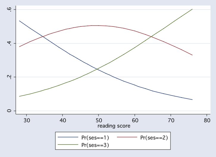
sort read
scatter p1 p2 p3 read, connect(l l l) msym(i i i)
 list read ses p1 p2 p3 if p1>p2, nolabel
+---------------------------------------------+
| read ses p1 p2 p3 |
|---------------------------------------------|
1. | 28 1 .5333536 .3807395 .0859069 |
2. | 31 2 .4899665 .4094642 .1005692 |
3. | 34 2 .4467301 .4358573 .1174126 |
4. | 34 2 .4467301 .4358573 .1174126 |
5. | 34 2 .4467301 .4358573 .1174126 |
|---------------------------------------------|
6. | 34 3 .4467301 .4358573 .1174126 |
7. | 34 1 .4467301 .4358573 .1174126 |
8. | 34 1 .4467301 .4358573 .1174126 |
+---------------------------------------------+
list read ses p1 p2 p3 if p1>p2 & p1>p3, nolabel
+---------------------------------------------+
| read ses p1 p2 p3 |
|---------------------------------------------|
1. | 28 1 .5333536 .3807395 .0859069 |
2. | 31 2 .4899665 .4094642 .1005692 |
3. | 34 2 .4467301 .4358573 .1174126 |
4. | 34 2 .4467301 .4358573 .1174126 |
5. | 34 2 .4467301 .4358573 .1174126 |
|---------------------------------------------|
6. | 34 3 .4467301 .4358573 .1174126 |
7. | 34 1 .4467301 .4358573 .1174126 |
8. | 34 1 .4467301 .4358573 .1174126 |
+---------------------------------------------+
drop p1 p2 p3
list read ses p1 p2 p3 if p1>p2, nolabel
+---------------------------------------------+
| read ses p1 p2 p3 |
|---------------------------------------------|
1. | 28 1 .5333536 .3807395 .0859069 |
2. | 31 2 .4899665 .4094642 .1005692 |
3. | 34 2 .4467301 .4358573 .1174126 |
4. | 34 2 .4467301 .4358573 .1174126 |
5. | 34 2 .4467301 .4358573 .1174126 |
|---------------------------------------------|
6. | 34 3 .4467301 .4358573 .1174126 |
7. | 34 1 .4467301 .4358573 .1174126 |
8. | 34 1 .4467301 .4358573 .1174126 |
+---------------------------------------------+
list read ses p1 p2 p3 if p1>p2 & p1>p3, nolabel
+---------------------------------------------+
| read ses p1 p2 p3 |
|---------------------------------------------|
1. | 28 1 .5333536 .3807395 .0859069 |
2. | 31 2 .4899665 .4094642 .1005692 |
3. | 34 2 .4467301 .4358573 .1174126 |
4. | 34 2 .4467301 .4358573 .1174126 |
5. | 34 2 .4467301 .4358573 .1174126 |
|---------------------------------------------|
6. | 34 3 .4467301 .4358573 .1174126 |
7. | 34 1 .4467301 .4358573 .1174126 |
8. | 34 1 .4467301 .4358573 .1174126 |
+---------------------------------------------+
drop p1 p2 p3
Here are some more of the Long & Freeze utilities.
prchange

ologit: Changes in Predicted Probabilities for ses

read
            Avg|Chg|         low      middle        high
Min->Max   .34431122  -.46714365  -.04932317   .51646684
   -+1/2   .00772587  -.00991599   -.0016728   .01158881
  -+sd/2   .07898068  -.10162368  -.01684734   .11847103
MargEfct   .00772609  -.00991603  -.00167311   .01158914

               low     middle       high
Pr(y|x)  .21930437  .50408369  .27661195

           read
    x=    52.23
sd(x)=  10.2529

prtab read

ologit: Predicted probabilities for ses

Predicted probability of outcome 1 (low)

----------------------
reading   |
score     | Prediction
----------+-----------
       28 |     0.5334
       31 |     0.4900
       34 |     0.4467
       35 |     0.4325
       36 |     0.4183
       37 |     0.4043
       39 |     0.3767
       41 |     0.3499
       42 |     0.3369
       43 |     0.3241
       44 |     0.3115
       45 |     0.2992
       46 |     0.2872
       47 |     0.2755
       48 |     0.2641
       50 |     0.2422
       52 |     0.2216
       53 |     0.2118
       54 |     0.2023
       55 |     0.1931
       57 |     0.1757
       60 |     0.1519
       61 |     0.1446
       63 |     0.1308
       65 |     0.1182
       66 |     0.1123
       68 |     0.1013
       71 |     0.0865
       73 |     0.0778
       76 |     0.0662
----------------------

Predicted probability of outcome 2 (middle)

----------------------
reading   |
score     | Prediction
----------+-----------
       28 |     0.3807
       31 |     0.4095
       34 |     0.4359
       35 |     0.4440
       36 |     0.4517
       37 |     0.4591
       39 |     0.4724
       41 |     0.4837
       42 |     0.4886
       43 |     0.4929
       44 |     0.4966
       45 |     0.4998
       46 |     0.5023
       47 |     0.5042
       48 |     0.5055
       50 |     0.5063
       52 |     0.5045
       53 |     0.5026
       54 |     0.5002
       55 |     0.4971
       57 |     0.4892
       60 |     0.4732
       61 |     0.4669
       63 |     0.4528
       65 |     0.4370
       66 |     0.4285
       68 |     0.4107
       71 |     0.3821
       73 |     0.3621
       76 |     0.3314
----------------------

Predicted probability of outcome 3 (high)

----------------------
reading   |
score     | Prediction
----------+-----------
       28 |     0.0859
       31 |     0.1006
       34 |     0.1174
       35 |     0.1235
       36 |     0.1300
       37 |     0.1366
       39 |     0.1509
       41 |     0.1663
       42 |     0.1745
       43 |     0.1830
       44 |     0.1919
       45 |     0.2010
       46 |     0.2105
       47 |     0.2202
       48 |     0.2304
       50 |     0.2515
       52 |     0.2740
       53 |     0.2856
       54 |     0.2976
       55 |     0.3098
       57 |     0.3351
       60 |     0.3749
       61 |     0.3886
       63 |     0.4164
       65 |     0.4448
       66 |     0.4591
       68 |     0.4880
       71 |     0.5314
       73 |     0.5601
       76 |     0.6024
----------------------

     read
x=  52.23
A Two Predictor Example
ologit ses read female

Iteration 0:   log likelihood = -210.58254
Iteration 1:   log likelihood = -200.28305
Iteration 2:   log likelihood = -200.18917
Iteration 3:   log likelihood = -200.18906

Ordered logit estimates                           Number of obs   =        200
                                                  LR chi2(2)      =      20.79
                                                  Prob > chi2     =     0.0000
Log likelihood = -200.18906                       Pseudo R2       =     0.0494

------------------------------------------------------------------------------
         ses |      Coef.   Std. Err.      z    P>|z|     [95% Conf. Interval]
-------------+----------------------------------------------------------------
        read |     .05714   .0138643     4.12   0.000     .0299665    .0843134
      female |  -.4195397   .2715105    -1.55   0.122    -.9516905    .1126111
-------------+----------------------------------------------------------------
       _cut1 |   1.477402   .7343098          (Ancillary parameters)
       _cut2 |   3.730551   .7791244
------------------------------------------------------------------------------

listcoef

ologit (N=200): Factor Change in Odds

  Odds of: >m vs <=m ---------------------------------------------------------------------- ses | b z P>|z|    e^b    e^bStdX      SDofX
-------------+--------------------------------------------------------
        read |   0.05714    4.121   0.000   1.0588   1.7965    10.2529
      female |  -0.41954   -1.545   0.122   0.6573   0.8110     0.4992
----------------------------------------------------------------------

fitstat

Measures of Fit for ologit of ses

Log-Lik Intercept Only:     -210.583     Log-Lik Full Model:         -200.189
D(196):                      400.378     LR(2):                        20.787
                                         Prob > LR:                     0.000
McFadden's R2:                 0.049     McFadden's Adj R2:             0.030
Maximum Likelihood R2:         0.099     Cragg & Uhler's R2:            0.112
McKelvey and Zavoina's R2:     0.108
Variance of y*:                3.690     Variance of error:             3.290
Count R2:                      0.500     Adj Count R2:                  0.048
AIC:                           2.042     AIC*n:                       408.378
BIC:                        -638.092     BIC':                        -10.190

prtab read female

ologit: Predicted probabilities for ses

Predicted probability of outcome 1 (low)

--------------------------
reading   |     female
score     |   male  female
----------+---------------
       28 | 0.4694  0.5737
       31 | 0.4270  0.5314
       34 | 0.3857  0.4885
       35 | 0.3723  0.4743
       36 | 0.3590  0.4601
       37 | 0.3460  0.4459
       39 | 0.3206  0.4179
       41 | 0.2962  0.3904
       42 | 0.2845  0.3769
       43 | 0.2730  0.3635
       44 | 0.2618  0.3504
       45 | 0.2509  0.3375
       46 | 0.2403  0.3249
       47 | 0.2300  0.3125
       48 | 0.2201  0.3003
       50 | 0.2011  0.2769
       52 | 0.1833  0.2546
       53 | 0.1749  0.2439
       54 | 0.1668  0.2335
       55 | 0.1591  0.2234
       57 | 0.1444  0.2042
       60 | 0.1244  0.1778
       61 | 0.1184  0.1696
       63 | 0.1069  0.1541
       65 | 0.0965  0.1398
       66 | 0.0916  0.1330
       68 | 0.0826  0.1204
       71 | 0.0705  0.1034
       73 | 0.0633  0.0933
       76 | 0.0539  0.0798
--------------------------

Predicted probability of outcome 2 (middle)

--------------------------
reading   |     female
score     |   male  female
----------+---------------
       28 | 0.4244  0.3539
       31 | 0.4494  0.3838
       34 | 0.4709  0.4124
       35 | 0.4772  0.4214
       36 | 0.4830  0.4302
       37 | 0.4883  0.4386
       39 | 0.4973  0.4544
       41 | 0.5040  0.4687
       42 | 0.5065  0.4751
       43 | 0.5084  0.4811
       44 | 0.5097  0.4866
       45 | 0.5103  0.4915
       46 | 0.5104  0.4959
       47 | 0.5098  0.4998
       48 | 0.5086  0.5030
       50 | 0.5044  0.5078
       52 | 0.4979  0.5102
       53 | 0.4937  0.5104
       54 | 0.4890  0.5100
       55 | 0.4838  0.5091
       57 | 0.4719  0.5053
       60 | 0.4505  0.4952
       61 | 0.4426  0.4907
       63 | 0.4257  0.4801
       65 | 0.4076  0.4675
       66 | 0.3982  0.4606
       68 | 0.3788  0.4454
       71 | 0.3487  0.4199
       73 | 0.3282  0.4014
       76 | 0.2977  0.3723
--------------------------

Predicted probability of outcome 3 (high)

--------------------------
reading   |     female
score     |   male  female
----------+---------------
       28 | 0.1062  0.0724
       31 | 0.1236  0.0848
       34 | 0.1433  0.0991
       35 | 0.1505  0.1043
       36 | 0.1580  0.1098
       37 | 0.1657  0.1155
       39 | 0.1821  0.1277
       41 | 0.1998  0.1410
       42 | 0.2090  0.1480
       43 | 0.2187  0.1554
       44 | 0.2286  0.1630
       45 | 0.2388  0.1710
       46 | 0.2493  0.1792
       47 | 0.2602  0.1878
       48 | 0.2713  0.1966
       50 | 0.2945  0.2153
       52 | 0.3188  0.2353
       53 | 0.3313  0.2457
       54 | 0.3441  0.2564
       55 | 0.3571  0.2675
       57 | 0.3838  0.2905
       60 | 0.4250  0.3270
       61 | 0.4391  0.3397
       63 | 0.4674  0.3658
       65 | 0.4959  0.3927
       66 | 0.5102  0.4064
       68 | 0.5387  0.4342
       71 | 0.5809  0.4767
       73 | 0.6084  0.5053
       76 | 0.6484  0.5480
--------------------------

      read  female
x=   52.23    .545
3-Category Predictor Example
tabulate prog, gen(prog)

    type of |
    program |      Freq.     Percent        Cum.
------------+-----------------------------------
    general |         45       22.50       22.50
   academic |        105       52.50       75.00
   vocation |         50       25.00      100.00
------------+-----------------------------------
      Total |        200      100.00

ologit ses prog1 prog2

Iteration 0:   log likelihood = -210.58254
Iteration 1:   log likelihood = -204.59144
Iteration 2:   log likelihood =   -204.554
Iteration 3:   log likelihood = -204.55398

Ordered logit estimates                           Number of obs   =        200
                                                  LR chi2(2)      =      12.06
                                                  Prob > chi2     =     0.0024
Log likelihood = -204.55398                       Pseudo R2       =     0.0286

------------------------------------------------------------------------------
         ses |      Coef.   Std. Err.      z    P>|z|     [95% Conf. Interval]
-------------+----------------------------------------------------------------
       prog1 |   -.180289    .382671    -0.47   0.638    -.9303103    .5697323
       prog2 |   .8500258   .3223129     2.64   0.008     .2183042    1.481747
-------------+----------------------------------------------------------------
       _cut1 |  -.8456498   .2679547          (Ancillary parameters)
       _cut2 |   1.335285   .2806444
------------------------------------------------------------------------------

test prog1 prog2
 ( 1)  prog1 = 0
 ( 2)  prog2 = 0

           chi2(  2) =   11.69
         Prob > chi2 =    0.0029
I prefer to use the academic group as the reference group and so will use prog1 and prog2 in the model.
ologit ses prog1 prog3

Iteration 0:   log likelihood = -210.58254
Iteration 1:   log likelihood = -204.59144
Iteration 2:   log likelihood =   -204.554
Iteration 3:   log likelihood = -204.55398

Ordered logit estimates                           Number of obs   =        200
                                                  LR chi2(2)      =      12.06
                                                  Prob > chi2     =     0.0024
Log likelihood = -204.55398                       Pseudo R2       =     0.0286

------------------------------------------------------------------------------
         ses |      Coef.   Std. Err.      z    P>|z|     [95% Conf. Interval]
-------------+----------------------------------------------------------------
       prog1 |  -1.030315   .3479667    -2.96   0.003    -1.712317   -.3483126
       prog3 |  -.8500258   .3223129    -2.64   0.008    -1.481747   -.2183042
-------------+----------------------------------------------------------------
       _cut1 |  -1.695676   .2334022          (Ancillary parameters)
       _cut2 |   .4852592    .195606
------------------------------------------------------------------------------

test prog1 prog3

 ( 1)  prog1 = 0
 ( 2)  prog3 = 0

           chi2(  2) =   11.69
         Prob > chi2 =    0.0029
Our Final Model: Three Predictors
ologit ses read female prog1 prog3

Iteration 0:   log likelihood = -210.58254
Iteration 1:   log likelihood = -197.79263
Iteration 2:   log likelihood = -197.63977
Iteration 3:   log likelihood = -197.63946

Ordered logit estimates                           Number of obs   =        200
                                                  LR chi2(4)      =      25.89
                                                  Prob > chi2     =     0.0000
Log likelihood = -197.63946                       Pseudo R2       =     0.0615

------------------------------------------------------------------------------
         ses |      Coef.   Std. Err.      z    P>|z|     [95% Conf. Interval]
-------------+----------------------------------------------------------------
        read |   .0481912   .0149969     3.21   0.001     .0187979    .0775846
      female |   -.444623   .2725877    -1.63   0.103    -.9788851    .0896391
       prog1 |  -.7946682   .3597171    -2.21   0.027    -1.499701   -.0896357
       prog3 |  -.4294622   .3493735    -1.23   0.219    -1.114222    .2552972
-------------+----------------------------------------------------------------
       _cut1 |    .682197   .8619888          (Ancillary parameters)
       _cut2 |   2.983569   .8891324
------------------------------------------------------------------------------

test prog1 prog3

 ( 1)  prog1 = 0
 ( 2)  prog3 = 0

           chi2(  2) =    5.04
         Prob > chi2 =    0.0803

listcoef

ologit (N=200): Factor Change in Odds

  Odds of: >m vs <=m ---------------------------------------------------------------------- ses | b z P>|z|    e^b    e^bStdX      SDofX
-------------+--------------------------------------------------------
        read |   0.04819    3.213   0.001   1.0494   1.6390    10.2529
      female |  -0.44462   -1.631   0.103   0.6411   0.8009     0.4992
       prog1 |  -0.79467   -2.209   0.027   0.4517   0.7170     0.4186
       prog3 |  -0.42946   -1.229   0.219   0.6509   0.8299     0.4341
----------------------------------------------------------------------

fitstat

Measures of Fit for ologit of ses

Log-Lik Intercept Only:     -210.583     Log-Lik Full Model:         -197.639
D(194):                      395.279     LR(4):                        25.886
                                         Prob > LR:                     0.000
McFadden's R2:                 0.061     McFadden's Adj R2:             0.033
Maximum Likelihood R2:         0.121     Cragg & Uhler's R2:            0.138
McKelvey and Zavoina's R2:     0.135
Variance of y*:                3.805     Variance of error:             3.290
Count R2:                      0.520     Adj Count R2:                  0.086
AIC:                           2.036     AIC*n:                       407.279
BIC:                        -632.595     BIC':                         -4.693

prchange

ologit: Changes in Predicted Probabilities for ses

read
            Avg|Chg|         low      middle        high
Min->Max   .28959884  -.38608418  -.04831406   .43439826
   -+1/2   .00633105  -.00808108  -.00141549   .00949657
  -+sd/2   .06479194    -.082848  -.01433992   .09718789
MargEfct   .00633115  -.00808108  -.00141564   .00949672

female
            Avg|Chg|         low      middle        high
    0->1   .05885413   .07370418   .01457703  -.08828117

prog1
            Avg|Chg|         low      middle        high
    0->1   .09951697   .14927547  -.00917467  -.14010078

prog3
            Avg|Chg|         low      middle        high
    0->1   .05353026   .07640016   .00389522  -.08029538

               low     middle       high
Pr(y|x)  .21309914  .51698065   .2699202

           read   female    prog1    prog3
    x=    52.23     .545     .225      .25
sd(x)=  10.2529   .49922   .41863  .434099

prtab read female, x(prog1=0 prog3=0)

ologit: Predicted probabilities for ses

Predicted probability of outcome 1 (low)

--------------------------
reading   |     female
score     |   male  female
----------+---------------
       28 | 0.3391  0.4446
       31 | 0.3075  0.4092
       34 | 0.2776  0.3748
       35 | 0.2681  0.3636
       36 | 0.2587  0.3525
       37 | 0.2496  0.3416
       39 | 0.2320  0.3202
       41 | 0.2152  0.2996
       42 | 0.2072  0.2896
       43 | 0.1994  0.2798
       44 | 0.1918  0.2702
       45 | 0.1845  0.2608
       46 | 0.1773  0.2516
       47 | 0.1704  0.2427
       48 | 0.1637  0.2339
       50 | 0.1509  0.2171
       52 | 0.1390  0.2011
       53 | 0.1333  0.1935
       54 | 0.1278  0.1861
       55 | 0.1226  0.1789
       57 | 0.1126  0.1652
       60 | 0.0989  0.1462
       61 | 0.0947  0.1403
       63 | 0.0868  0.1291
       65 | 0.0794  0.1186
       66 | 0.0760  0.1137
       68 | 0.0695  0.1043
       71 | 0.0607  0.0916
       73 | 0.0554  0.0839
       76 | 0.0483  0.0734
--------------------------

Predicted probability of outcome 2 (middle)

--------------------------
reading   |     female
score     |   male  female
----------+---------------
       28 | 0.4976  0.4442
       31 | 0.5085  0.4645
       34 | 0.5157  0.4821
       35 | 0.5173  0.4873
       36 | 0.5184  0.4922
       37 | 0.5190  0.4966
       39 | 0.5191  0.5045
       41 | 0.5173  0.5107
       42 | 0.5158  0.5132
       43 | 0.5139  0.5153
       44 | 0.5115  0.5169
       45 | 0.5087  0.5181
       46 | 0.5055  0.5189
       47 | 0.5019  0.5193
       48 | 0.4979  0.5192
       50 | 0.4888  0.5176
       52 | 0.4782  0.5144
       53 | 0.4724  0.5121
       54 | 0.4663  0.5094
       55 | 0.4599  0.5063
       57 | 0.4463  0.4988
       60 | 0.4241  0.4848
       61 | 0.4163  0.4795
       63 | 0.4001  0.4677
       65 | 0.3834  0.4548
       66 | 0.3749  0.4479
       68 | 0.3577  0.4334
       71 | 0.3315  0.4101
       73 | 0.3141  0.3937
       76 | 0.2882  0.3683
--------------------------

Predicted probability of outcome 3 (high)

--------------------------
reading   |     female
score     |   male  female
----------+---------------
       28 | 0.1633  0.1112
       31 | 0.1840  0.1263
       34 | 0.2067  0.1431
       35 | 0.2147  0.1491
       36 | 0.2229  0.1553
       37 | 0.2314  0.1618
       39 | 0.2490  0.1753
       41 | 0.2674  0.1896
       42 | 0.2770  0.1972
       43 | 0.2867  0.2049
       44 | 0.2967  0.2129
       45 | 0.3068  0.2210
       46 | 0.3172  0.2295
       47 | 0.3277  0.2381
       48 | 0.3384  0.2469
       50 | 0.3603  0.2653
       52 | 0.3828  0.2845
       53 | 0.3943  0.2944
       54 | 0.4058  0.3045
       55 | 0.4175  0.3148
       57 | 0.4411  0.3360
       60 | 0.4770  0.3690
       61 | 0.4890  0.3802
       63 | 0.5131  0.4032
       65 | 0.5371  0.4266
       66 | 0.5491  0.4384
       68 | 0.5728  0.4623
       71 | 0.6078  0.4983
       73 | 0.6305  0.5224
       76 | 0.6635  0.5583
--------------------------

      read  female   prog1   prog3
x=   52.23    .545       0       0
Using linktest to test for model specification errors.
linktest

Iteration 0:   log likelihood = -210.58254
Iteration 1:   log likelihood = -197.64558
Iteration 2:   log likelihood = -197.49272
Iteration 3:   log likelihood = -197.49241

Ordered logit estimates                           Number of obs   =        200
                                                  LR chi2(2)      =      26.18
                                                  Prob > chi2     =     0.0000
Log likelihood = -197.49241                       Pseudo R2       =     0.0622

------------------------------------------------------------------------------
         ses |      Coef.   Std. Err.      z    P>|z|     [95% Conf. Interval]
-------------+----------------------------------------------------------------
        _hat |   .4784934   .9824955     0.49   0.626    -1.447162    2.404149
      _hatsq |   .1304895    .241209     0.54   0.589    -.3422715    .6032505
-------------+----------------------------------------------------------------
       _cut1 |   .2243895   .9347503          (Ancillary parameters)
       _cut2 |   2.526304   .9591539
------------------------------------------------------------------------------
Here again is the test of proportional odds.
omodel logit ses read female prog1 prog3

Iteration 0:   log likelihood = -210.58254
Iteration 1:   log likelihood = -197.79263
Iteration 2:   log likelihood = -197.63977
Iteration 3:   log likelihood = -197.63946

Ordered logit estimates                           Number of obs   =        200
                                                  LR chi2(4)      =      25.89
                                                  Prob > chi2     =     0.0000
Log likelihood = -197.63946                       Pseudo R2       =     0.0615

------------------------------------------------------------------------------
         ses |      Coef.   Std. Err.      z    P>|z|     [95% Conf. Interval]
-------------+----------------------------------------------------------------
        read |   .0481912   .0149969     3.21   0.001     .0187979    .0775846
      female |   -.444623   .2725877    -1.63   0.103    -.9788851    .0896391
       prog1 |  -.7946682   .3597171    -2.21   0.027    -1.499701   -.0896357
       prog3 |  -.4294622   .3493735    -1.23   0.219    -1.114222    .2552972
-------------+----------------------------------------------------------------
       _cut1 |    .682197   .8619888          (Ancillary parameters)
       _cut2 |   2.983569   .8891324
------------------------------------------------------------------------------

Approximate likelihood-ratio test of proportionality of odds
across response categories:
         chi2(4) =      6.46
       Prob > chi2 =    0.1676
Let’s look at the generalized ordered logistic model.
gologit ses read female prog1 prog3
Iteration 0:  Log Likelihood = -210.58254
Iteration 1:  Log Likelihood = -194.98035
Iteration 2:  Log Likelihood = -194.40757
Iteration 3:  Log Likelihood = -194.40633
Iteration 4:  Log Likelihood = -194.40633

Generalized Ordered Logit Estimates                 Number of obs    =     200
                                                    Model chi2(8)    =   32.35
                                                    Prob > chi2      =  0.0001
Log Likelihood =   -194.4063269                     Pseudo R2        =  0.0768

------------------------------------------------------------------------------
         ses |      Coef.   Std. Err.      z    P>|z|     [95% Conf. Interval]
-------------+----------------------------------------------------------------
mleq1        |
        read |    .053024   .0209806     2.53   0.011     .0119028    .0941451
      female |  -.7215625   .3628111    -1.99   0.047    -1.432659   -.0104659
       prog1 |  -.6979021   .4224733    -1.65   0.099    -1.525934    .1301303
       prog3 |   .1012859   .4606329     0.22   0.826    -.8015381     1.00411
       _cons |  -.9279434   1.173037    -0.79   0.429    -3.227054    1.371167
-------------+----------------------------------------------------------------
mleq2        |
        read |   .0452445   .0176378     2.57   0.010     .0106751     .079814
      female |  -.2204975   .3273852    -0.67   0.501    -.8621607    .4211657
       prog1 |   -.745496   .4380499    -1.70   0.089    -1.604058     .113066
       prog3 |  -1.029291   .4782148    -2.15   0.031    -1.966575   -.0920073
       _cons |  -2.836412   1.042437    -2.72   0.007    -4.879551   -.7932731
------------------------------------------------------------------------------

test [mleq1=mleq2]

 ( 1)  [mleq1]read - [mleq2]read = 0
 ( 2)  [mleq1]female - [mleq2]female = 0
 ( 3)  [mleq1]prog1 - [mleq2]prog1 = 0
 ( 4)  [mleq1]prog3 - [mleq2]prog3 = 0

           chi2(  4) =    5.91
         Prob > chi2 =    0.2056