- Background for Survival Analysis
- The UIS data
- Exploring the data: Univariate Analyses
- Model Building
- Interactions
- Proportionality Assumption
- Graphing Survival Functions from stcox command
- Goodness of Fit of the Final Model
The Stata program on which the seminar is based. The UIS_small data file for the seminar.
Background for Survival Analysis
The goal of this seminar is to give a brief introduction to the topic of survival analysis. We will be using a smaller and slightly modified version of the UIS data set from the book “Applied Survival Analysis” by Hosmer and Lemeshow. We strongly encourage everyone who is interested in learning survival analysis to read this text as it is a very good and thorough introduction to the topic.
Survival analysis is just another name for time to event analysis. The term survival analysis is predominately used in biomedical sciences where the interest is in observing time to death either of patients or of laboratory animals. Time to event analysis has also been used widely in the social sciences where interest is on analyzing time to events such as job changes, marriage, birth of children and so forth. The engineering sciences have also contributed to the development of survival analysis which is called “reliability analysis” or “failure time analysis” in this field since the main focus is in modeling the time it takes for machines or electronic components to break down. The developments from these diverse fields have for the most part been consolidated into the field of “survival analysis”. For more background please refer to the excellent discussion in Chapter 1 of Event History Analysis by Paul Allison.
There are certain aspects of survival analysis data, such as censoring and non-normality, that generate great difficulty when trying to analyze the data using traditional statistical models such as multiple linear regression. The non-normality aspect of the data violates the normality assumption of most commonly used statistical model such as regression or ANOVA, etc. A censored observation is defined as an observation with incomplete information. There are four different types of censoring possible: right truncation, left truncation, right censoring and left censoring. We will focus exclusively on right censoring for a number of reasons. Most data used in analyses have only right censoring. Furthermore, right censoring is the most easily understood of all the four types of censoring and if a researcher can understand the concept of right censoring thoroughly it becomes much easier to understand the other three types. When an observation is right censored it means that the information is incomplete because the subject did not have an event during the time that the subject was part of the study. The point of survival analysis is to follow subjects over time and observe at which point in time they experience the event of interest. It often happens that the study does not span enough time in order to observe the event for all the subjects in the study. This could be due to a number of reasons. Perhaps subjects drop out of the study for reasons unrelated to the study (i.e. patients moving to another area and leaving no forwarding address). The common feature of all of these examples is that if the subject had been able to stay in the study then it would have been possible to observe the time of the event eventually.
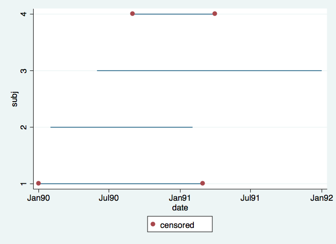
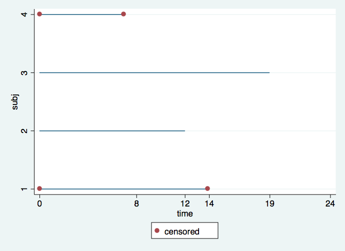
It is important to understand the difference between calendar time and time in the study. It is very common for subjects to enter the study continuously throughout the length of the study. This situation is reflected in the first graph where we can see the staggered entry of four subjects. Red dots denote intervals in which the event is censored, whereas intervals without red dots signify that the event occurred. It would appear that subject 4 dropped out after only a short time (hit by a bus, very tragic) and that subject 3 did not experience an event by the time the study ended but if the study had gone on longer (had more funding) we would have known the time when this subject would have experienced an event.
clear
input subj tp censored str11 datestr
1 1 0 "1 jan 1990"
1 2 0 "1 mar 1991"
2 1 1 "1 feb 1990"
2 2 1 "1 feb 1991"
3 1 1 "1 jun 1990"
3 2 1 "31 dec 1991"
4 1 0 "1 sep 1990"
4 2 0 "1 apr 1991"
end

gen date = date(datestr, "DMY")
format date %dmy
twoway (line subj date, connect(L))(scatter subj date if censored==0), ///
       ylabel(1 2 3 4) legend(order (2 "censored"))

gen time =0 if tp==1
replace time= (date-date[_n-1])/30.5 if tp==2
twoway (line subj time, connect(L))(scatter subj time if censored==0), ///
       ylabel(1 2 3 4) legend(order (2 "censored")) xlabel(0 8 12 14 19 24)
The other important concept in survival analysis is the hazard rate. From looking at data with discrete time (time measured in large intervals such as month, years or even decades) we can get an intuitive idea of the hazard rate. For discrete time the hazard rate is the probability that an individual will experience an event at time t while that individual is at risk for having an event. Thus, the hazard rate is really just the unobserved rate at which events occur. If the hazard rate is constant over time and it was equal to 1.5 for example this would mean that one would expect 1.5 events to occur in a time interval that is one unit long. Furthermore, if a person had a hazard rate of 1.2 at time t and a second person had a hazard rate of 2.4 at time t then it would be correct to say that the second person’s risk of an event would be two times greater at time t. It is important to realize that the hazard rate is an un-observed variable yet it controls both the occurrence and the timing of the events. It is the fundamental dependent variable in survival analysis.
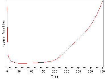
Another important aspect of the hazard function is to understand how the shape of the hazard function will influence the other variables of interest such as the survival function. The first graph below illustrates a hazard function with a ‘bathtub shape’. This graph is depicting the hazard function for the survival of organ transplant patients. At time equal to zero they are having the transplant and since this is a very dangerous operation they have a very high hazard (a great chance of dying). The first 10 days after the operation are also very dangerous with a high chance of the patient dying but the danger is less than during the actual operation and hence the hazard is decrease during this period. If the patient has survived past day 10 then they are in very good shape and have a very little chance of dying in the following 6 months. After 6 months the patients begin to experience deterioration and the chances of dying increase again and therefore the hazard function starts to increase. After one year almost all patients are dead and hence the very high hazard function which will continue to increase.
The hazard function may not seem like an exciting variable to model but other indicators of interest, such as the survival function, are derived from the hazard rate. Once we have modeled the hazard rate we can easily obtain these other functions of interest. To summarize, it is important to understand the concept of the hazard function and to understand the shape of the hazard function.
An example of a hazard function for heart transplant patients.
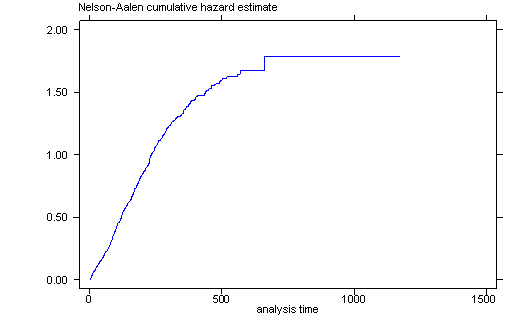
We are generally unable to generate the hazard function instead we usually look at the cumulative hazard curve.
use https://stats.idre.ucla.edu/stat/data/uis.dta, clear
gen id = ID
drop ID
stset time, failure(censor)
sts graph, na
The UIS data
The goal of the UIS data is to model time until return to drug use for patients enrolled in two different residential treatment programs that differed in length (treat=0 is the short program and treat=1 is the long program). The patients were randomly assigned to two different sites (site=0 is site A and site=1 is site B). The variable age indicates age at enrollment, herco indicates heroin or cocaine use in the past three months (herco=1 indicates heroin and cocaine use, herco=2 indicates either heroin or cocaine use and herco=3 indicates neither heroin nor cocaine use) and ndrugtx indicates the number of previous drug treatments. The variables time contains the time until return to drug use and the censor variable indicates whether the subject returned to drug use (censor=1 indicates return to drug use and censor=0 otherwise).
Let’s look at the first 10 observations of the UIS data set. Note that subject 5 is censored and did not experience an event while in the study. Also note that the coding for censor is rather counter-intuitive since the value 1 indicates an event and 0 indicates censoring. It would perhaps be more appropriate to call this variable “event”.
list id time censor age ndrugtx treat site herco in 1/10, nodisplay


            id       time     censor        age    ndrugtx      treat       site      herco
  1.         1        188          1         39          1          1          0          3
  2.         2         26          1         33          8          1          0          3
  3.         3        207          1         33          3          1          0          2
  4.         4        144          1         32          1          0          0          3
  5.         5        551          0         24          5          1          0          2
  6.         6         32          1         30          1          1          0          1
  7.         7        459          1         39         34          1          0          3
  8.         8         22          1         27          2          1          0          3
  9.         9        210          1         40          3          1          0          2
 10.        10        184          1         36          7          1          0          2
Exploring the data: Univariate Analyses
In any data analysis it is always a great idea to do some univariate analysis before proceeding to more complicated models. In survival analysis it is highly recommended to look at the Kaplan-Meier curves for all the categorical predictors. This will provide insight into the shape of the survival function for each group and give an idea of whether or not the groups are proportional (i.e. the survival functions are approximately parallel). We also consider the tests of equality across strata to explore whether or not to include the predictor in the final model. For the categorical variables we will use the log-rank test of equality across strata which is a non-parametric test. For the continuous variables we will use a univariate Cox proportional hazard regression which is a semi-parametric model. We will consider including the predictor if the test has a p-value of 0.2 – 0.25 or less. We are using this elimination scheme because all the predictors in the data set are variables that could be relevant to the model. If the predictor has a p-value greater than 0.25 in a univariate analysis it is highly unlikely that it will contribute anything to a model which includes other predictors.
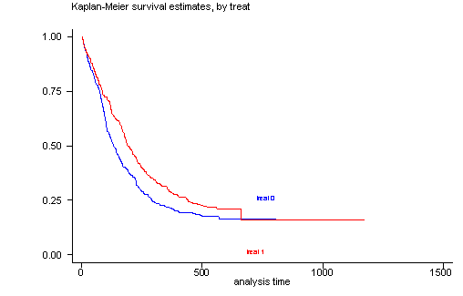
The log-rank test of equality across strata for the predictor treat has a p-value of 0.0091, thus treat will be included a potential candidate for the final model. From the graph we see that the survival function for each group of treat are not perfectly parallel but separate except at the very beginning and at the very end. The overlap at the very end should not cause too much concern because it is determined by only a very few number of censored subjects out of a sample with 628 subjects. In general, the log-rank test places the more emphasis on differences in the curves at larger time values. This is why we get such a small p-value even though the two survival curves appear to be very close together for time less than 100 days.
sts test treat, logrank
sts graph, by(treat)

         failure _d:  censor
   analysis time _t:  time

Log-rank test for equality of survivor functions

      |   Events         Events
treat |  observed       expected
------+-------------------------
0     |       265         235.80
1     |       243         272.20
------+-------------------------
Total |       508         508.00

            chi2(1) =       6.80
            Pr>chi2 =     0.0091
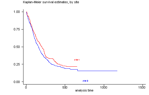
The log-rank test of equality across strata for the predictor site has a p-value of 0.1240, thus site will be included as a potential candidate for the final model because this p-value is still less than our cut-off of 0.2. From the graph we see that the survival curves are not all that parallel and that there are two periods ( [0, 100] and [200, 300] ) where the curves are very close together. This would explain the rather high p-value from the log-rank test.
sts test site, logrank
sts graph, by(site)

         failure _d:  censor
   analysis time _t:  time

Log-rank test for equality of survivor functions

      |   Events         Events
site  |  observed       expected
------+-------------------------
0     |       364         347.94
1     |       144         160.06
------+-------------------------
Total |       508         508.00

            chi2(1) =       2.37
            Pr>chi2 =     0.1240
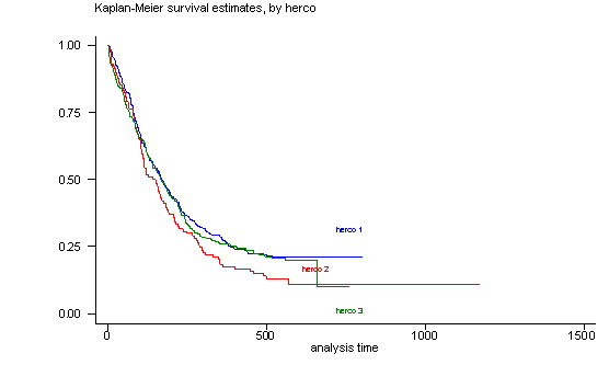
The log-rank test of equality across strata for the predictor herco has a p-value of 0.1473, thus herco will be included as potential candidate for the final model. From the graph we see that the three groups are not parallel and that especially the groups herco=1 and herco=3 overlap for most of the graph. This lack of parallelism could pose a problem when we include this predictor in the Cox proportional hazard model since one of the assumptions is proportionality of the predictors.
sts test herco
sts graph, by(herco) noborder

         failure _d:  censor
   analysis time _t:  time

Log-rank test for equality of survivor functions

      |   Events         Events
herco |  observed       expected
------+-------------------------
1     |       228         242.14
2     |       100          84.19
3     |       180         181.67
------+-------------------------
Total |       508         508.00

            chi2(2) =       3.83
            Pr>chi2 =     0.1473
It is not feasible to calculate a Kaplan-Meier curve for the continuous predictors since there would be a curve for each level of the predictor and a continuous predictor simply has too many different levels. Instead we consider the Cox proportional hazard model with a single continuous predictor. Unfortunately it is not possibly to produce a plot when using the stcox command. Instead we consider the Chi-squared test for ndrugtx which has a p-value of 0.0003 thus ndrugtx is a potential candidate for the final model since the p-value is less than our cut-off value of 0.2. We specify the option nohr to indicate that we do not want to see the hazard ratio rather we want to look at the coefficients.
stcox ndrugtx, nohr

Cox regression -- Breslow method for ties

No. of subjects =          611                     Number of obs   =       611
No. of failures =          496
Time at risk    =       143002
                                                   LR chi2(1)      =     13.35
Log likelihood  =    -2868.299                     Prob > chi2     =    0.0003
------------------------------------------------------------------------------
          _t |
          _d |      Coef.   Std. Err.      z    P>|z|     [95% Conf. Interval]
-------------+----------------------------------------------------------------
     ndrugtx |    .029372   .0074979     3.92   0.000     .0146763    .0440676
------------------------------------------------------------------------------
In this model the Chi-squared test of age also has a p-value of less than 0.2 and so it is a potential candidate for the final model.
stcox age, nohr

Cox regression -- Breslow method for ties

No. of subjects =          623                     Number of obs   =       623
No. of failures =          504
Time at risk    =       146816
                                                   LR chi2(1)      =      3.24
Log likelihood  =   -2931.4929                     Prob > chi2     =    0.0719
------------------------------------------------------------------------------
          _t |
          _d |      Coef.   Std. Err.      z    P>|z|     [95% Conf. Interval]
-------------+----------------------------------------------------------------
         age |  -.0128641   .0071888    -1.79   0.074    -.0269539    .0012256
------------------------------------------------------------------------------
Model Building
For our model building, we will first consider the model which will include all the predictors that had a p-value of less than 0.2 – 0.25 in the univariate analyses which in this particular analysis means that we will include every predictor in our model. The categorical predictor herco has three levels and therefore we will include this predictor using dummy variable with the group herco=1 as the reference group. We can create these dummy variables on the fly by using the xi command with stcox.
stcox age ndrugtx i.treat i.site i.herco, nohr

         failure _d:  censor
   analysis time _t:  time

Iteration 0:   log likelihood =  -2868.555
Iteration 1:   log likelihood = -2851.6989
Iteration 2:   log likelihood = -2851.0884
Iteration 3:   log likelihood = -2851.0863
Refining estimates:
Iteration 0:   log likelihood = -2851.0863

Cox regression -- Breslow method for ties

No. of subjects =          610                     Number of obs   =       610
No. of failures =          495
Time at risk    =       142994
                                                   LR chi2(6)      =     34.94
Log likelihood  =   -2851.0863                     Prob > chi2     =    0.0000

------------------------------------------------------------------------------
          _t |      Coef.   Std. Err.      z    P>|z|     [95% Conf. Interval]
-------------+----------------------------------------------------------------
         age |  -.0237543   .0075611    -3.14   0.002    -.0385737   -.0089349
     ndrugtx |    .034745   .0077538     4.48   0.000     .0195478    .0499422
     1.treat |  -.2540169    .091005    -2.79   0.005    -.4323834   -.0756504
      1.site |  -.1723881   .1020981    -1.69   0.091    -.3724966    .0277205
             |
       herco |
          2  |   .2467753   .1227597     2.01   0.044     .0061706    .4873799
          3  |    .125668   .1030729     1.22   0.223    -.0763513    .3276873
------------------------------------------------------------------------------

test 2.herco 3.herco

 ( 1)  2.herco = 0
 ( 2)  3.herco = 0

           chi2(  2) =    4.36
         Prob > chi2 =    0.1130
The predictor herco is clearly not significant and we will drop it from the final model. The predictor site is also not significant but from prior research we know that this is a very important variable to have in the final model and therefore we will not eliminate site from the model. So, the final model of main effects include: age, ndrugtx, treat and site.
stcox age ndrugtx i.treat i.site, nohr

         failure _d:  censor
   analysis time _t:  time

Iteration 0:   log likelihood =  -2868.555
Iteration 1:   log likelihood = -2853.8641
Iteration 2:   log likelihood = -2853.2393
Iteration 3:   log likelihood = -2853.2371
Refining estimates:
Iteration 0:   log likelihood = -2853.2371

Cox regression -- Breslow method for ties

No. of subjects =          610                     Number of obs   =       610
No. of failures =          495
Time at risk    =       142994
                                                   LR chi2(4)      =     30.64
Log likelihood  =   -2853.2371                     Prob > chi2     =    0.0000

------------------------------------------------------------------------------
          _t |      Coef.   Std. Err.      z    P>|z|     [95% Conf. Interval]
-------------+----------------------------------------------------------------
         age |  -.0221289   .0075108    -2.95   0.003    -.0368499    -.007408
     ndrugtx |   .0350249   .0076676     4.57   0.000     .0199967     .050053
     1.treat |  -.2436784   .0905411    -2.69   0.007    -.4211358   -.0662211
      1.site |  -.1683325   .1004119    -1.68   0.094    -.3651362    .0284712
------------------------------------------------------------------------------
Interactions
Next we need to consider interactions. We do not have any prior knowledge of specific interactions that we must include so we will consider all the possible interactions. Since our model is rather small this is manageable but the ideal situation is when all model building, including interactions, are theory driven.
The interaction term of age with ndrugtx is not significant and will not be included in the model.
stcox age ndrugtx i.treat i.site c.age#c.ndrug, nohr

         failure _d:  censor
   analysis time _t:  time

Iteration 0:   log likelihood =  -2868.555
Iteration 1:   log likelihood = -2854.6056
Iteration 2:   log likelihood = -2851.8845
Iteration 3:   log likelihood = -2851.8195
Iteration 4:   log likelihood = -2851.8195
Refining estimates:
Iteration 0:   log likelihood = -2851.8195

Cox regression -- Breslow method for ties

No. of subjects =          610                     Number of obs   =       610
No. of failures =          495
Time at risk    =       142994
                                                   LR chi2(5)      =     33.47
Log likelihood  =   -2851.8195                     Prob > chi2     =    0.0000

------------------------------------------------------------------------------
          _t |      Coef.   Std. Err.      z    P>|z|     [95% Conf. Interval]
-------------+----------------------------------------------------------------
         age |  -.0110172   .0100068    -1.10   0.271    -.0306302    .0085959
     ndrugtx |   .1054144   .0419532     2.51   0.012     .0231875    .1876412
     1.treat |  -.2352811   .0906447    -2.60   0.009    -.4129416   -.0576207
      1.site |  -.1746173   .1004498    -1.74   0.082    -.3714953    .0222607
             |
       c.age#|
   c.ndrugtx |  -.0020967   .0012469    -1.68   0.093    -.0045406    .0003472
------------------------------------------------------------------------------
The interaction age and treat is not significant and will not be included in the model.
stcox age ndrugtx i.treat i.site c.age#i.treat, nohr


         failure _d:  censor
   analysis time _t:  time

Iteration 0:   log likelihood =  -2868.555
Iteration 1:   log likelihood =  -2852.845
Iteration 2:   log likelihood = -2852.1654
Iteration 3:   log likelihood = -2852.1631
Refining estimates:
Iteration 0:   log likelihood = -2852.1631

Cox regression -- Breslow method for ties

No. of subjects =          610                     Number of obs   =       610
No. of failures =          495
Time at risk    =       142994
                                                   LR chi2(5)      =     32.78
Log likelihood  =   -2852.1631                     Prob > chi2     =    0.0000

------------------------------------------------------------------------------
          _t |      Coef.   Std. Err.      z    P>|z|     [95% Conf. Interval]
-------------+----------------------------------------------------------------
         age |  -.0114621   .0103995    -1.10   0.270    -.0318448    .0089205
     ndrugtx |   .0357659   .0077155     4.64   0.000     .0206437     .050888
     1.treat |   .4483383   .4809163     0.93   0.351    -.4942403    1.390917
      1.site |  -.1492698   .1010768    -1.48   0.140    -.3473766     .048837
             |
 treat#c.age |
          1  |   -.021469   .0146588    -1.46   0.143    -.0501996    .0072616
------------------------------------------------------------------------------
The interaction age anf site is significant and will be included in the model.
stcox age ndrugtx i.treat i.site c.age#i.site, nohr

         failure _d:  censor
   analysis time _t:  time

Iteration 0:   log likelihood =  -2868.555
Iteration 1:   log likelihood =  -2851.487
Iteration 2:   log likelihood = -2850.8935
Iteration 3:   log likelihood = -2850.8915
Refining estimates:
Iteration 0:   log likelihood = -2850.8915

Cox regression -- Breslow method for ties

No. of subjects =          610                     Number of obs   =       610
No. of failures =          495
Time at risk    =       142994
                                                   LR chi2(5)      =     35.33
Log likelihood  =   -2850.8915                     Prob > chi2     =    0.0000

------------------------------------------------------------------------------
          _t |      Coef.   Std. Err.      z    P>|z|     [95% Conf. Interval]
-------------+----------------------------------------------------------------
         age |  -.0336943   .0092913    -3.63   0.000     -.051905   -.0154837
     ndrugtx |   .0364537   .0077012     4.73   0.000     .0213597    .0515478
     1.treat |  -.2674113   .0912282    -2.93   0.003    -.4462153   -.0886073
      1.site |  -1.245928   .5087349    -2.45   0.014     -2.24303   -.2488262
             |
  site#c.age |
          1  |   .0337728   .0155087     2.18   0.029     .0033764    .0641693
------------------------------------------------------------------------------
The interaction drug anf treat is not significant and will be not included in the model.
stcox age ndrugtx i.treat i.site c.ndrug#i.treat, nohr

         failure _d:  censor
   analysis time _t:  time

Iteration 0:   log likelihood =  -2868.555
Iteration 1:   log likelihood = -2854.1019
Iteration 2:   log likelihood = -2853.0275
Iteration 3:   log likelihood = -2853.0174
Iteration 4:   log likelihood = -2853.0174
Refining estimates:
Iteration 0:   log likelihood = -2853.0174

Cox regression -- Breslow method for ties

No. of subjects =          610                     Number of obs   =       610
No. of failures =          495
Time at risk    =       142994
                                                   LR chi2(5)      =     31.08
Log likelihood  =   -2853.0174                     Prob > chi2     =    0.0000

------------------------------------------------------------------------------
          _t |      Coef.   Std. Err.      z    P>|z|     [95% Conf. Interval]
-------------+----------------------------------------------------------------
         age |  -.0220158   .0075029    -2.93   0.003    -.0367212   -.0073105
     ndrugtx |   .0404798    .011066     3.66   0.000     .0187909    .0621686
     1.treat |  -.1949252   .1166714    -1.67   0.095     -.423597    .0337465
      1.site |  -.1708522   .1004592    -1.70   0.089    -.3677487    .0260442
             |
       treat#|
   c.ndrugtx |
          1  |  -.0099061   .0149405    -0.66   0.507    -.0391889    .0193767
------------------------------------------------------------------------------
The interaction drug and site is not significant and will not be included in the model.
stcox age ndrugtx i.treat i.site c.ndrug#i.site, nohr


         failure _d:  censor
   analysis time _t:  time

Iteration 0:   log likelihood =  -2868.555
Iteration 1:   log likelihood = -2853.9255
Iteration 2:   log likelihood = -2853.1789
Iteration 3:   log likelihood = -2853.1746
Iteration 4:   log likelihood = -2853.1746
Refining estimates:
Iteration 0:   log likelihood = -2853.1746

Cox regression -- Breslow method for ties

No. of subjects =          610                     Number of obs   =       610
No. of failures =          495
Time at risk    =       142994
                                                   LR chi2(5)      =     30.76
Log likelihood  =   -2853.1746                     Prob > chi2     =    0.0000

------------------------------------------------------------------------------
          _t |      Coef.   Std. Err.      z    P>|z|     [95% Conf. Interval]
-------------+----------------------------------------------------------------
         age |  -.0222734   .0075266    -2.96   0.003    -.0370251   -.0075216
     ndrugtx |   .0366438   .0088665     4.13   0.000     .0192658    .0540218
     1.treat |  -.2454197   .0906816    -2.71   0.007    -.4231524    -.067687
      1.site |  -.1417165   .1253391    -1.13   0.258    -.3873766    .1039435
             |
        site#|
   c.ndrugtx |
          1  |  -.0059702   .0169939    -0.35   0.725    -.0392776    .0273373
------------------------------------------------------------------------------
The interaction treat and site is not significant and will not be included in the model.
stcox age ndrugtx i.treat i.site i.treat#i.site, nohr

         failure _d:  censor
   analysis time _t:  time

Iteration 0:   log likelihood =  -2868.555
Iteration 1:   log likelihood = -2852.4136
Iteration 2:   log likelihood = -2851.8662
Iteration 3:   log likelihood = -2851.8645
Refining estimates:
Iteration 0:   log likelihood = -2851.8645

Cox regression -- Breslow method for ties

No. of subjects =          610                     Number of obs   =       610
No. of failures =          495
Time at risk    =       142994
                                                   LR chi2(5)      =     33.38
Log likelihood  =   -2851.8645                     Prob > chi2     =    0.0000

------------------------------------------------------------------------------
          _t |      Coef.   Std. Err.      z    P>|z|     [95% Conf. Interval]
-------------+----------------------------------------------------------------
         age |  -.0238596    .007638    -3.12   0.002    -.0388297   -.0088895
     ndrugtx |   .0361507   .0077457     4.67   0.000     .0209694    .0513321
     1.treat |  -.3404088    .107682    -3.16   0.002    -.5514616    -.129356
      1.site |  -.3238557    .139417    -2.32   0.020     -.597108   -.0506033
             |
  treat#site |
        1 1  |   .3335144   .2009322     1.66   0.097    -.0603054    .7273342
------------------------------------------------------------------------------
The final model including interaction. Now we can see why it was important to include site in our model as prior research had suggested because it turns out that site is involved in the only significant interaction in the model. We can compare the model with the interaction to the model without the interaction using the lrtest command since the models are nested. The significant lrtest indicates that we reject the null hypothesis that the two models fit the data equally well and conclude that the bigger model with the interaction fits the data better than the smaller model which did not include the interaction.
stcox age ndrugtx i.treat i.site c.age#i.site, nohr

         failure _d:  censor
   analysis time _t:  time

Iteration 0:   log likelihood =  -2868.555
Iteration 1:   log likelihood =  -2851.487
Iteration 2:   log likelihood = -2850.8935
Iteration 3:   log likelihood = -2850.8915
Refining estimates:
Iteration 0:   log likelihood = -2850.8915

Cox regression -- Breslow method for ties

No. of subjects =          610                     Number of obs   =       610
No. of failures =          495
Time at risk    =       142994
                                                   LR chi2(5)      =     35.33
Log likelihood  =   -2850.8915                     Prob > chi2     =    0.0000

------------------------------------------------------------------------------
          _t |      Coef.   Std. Err.      z    P>|z|     [95% Conf. Interval]
-------------+----------------------------------------------------------------
         age |  -.0336943   .0092913    -3.63   0.000     -.051905   -.0154837
     ndrugtx |   .0364537   .0077012     4.73   0.000     .0213597    .0515478
     1.treat |  -.2674113   .0912282    -2.93   0.003    -.4462153   -.0886073
      1.site |  -1.245928   .5087349    -2.45   0.014     -2.24303   -.2488262
             |
  site#c.age |
          1  |   .0337728   .0155087     2.18   0.029     .0033764    .0641693
------------------------------------------------------------------------------

estimates store m1

stcox age ndrugtx i.treat i.site, nohr

         failure _d:  censor
   analysis time _t:  time

Iteration 0:   log likelihood =  -2868.555
Iteration 1:   log likelihood = -2853.8641
Iteration 2:   log likelihood = -2853.2393
Iteration 3:   log likelihood = -2853.2371
Refining estimates:
Iteration 0:   log likelihood = -2853.2371

Cox regression -- Breslow method for ties

No. of subjects =          610                     Number of obs   =       610
No. of failures =          495
Time at risk    =       142994
                                                   LR chi2(4)      =     30.64
Log likelihood  =   -2853.2371                     Prob > chi2     =    0.0000

------------------------------------------------------------------------------
          _t |      Coef.   Std. Err.      z    P>|z|     [95% Conf. Interval]
-------------+----------------------------------------------------------------
         age |  -.0221289   .0075108    -2.95   0.003    -.0368499    -.007408
     ndrugtx |   .0350249   .0076676     4.57   0.000     .0199967     .050053
     1.treat |  -.2436784   .0905411    -2.69   0.007    -.4211358   -.0662211
      1.site |  -.1683325   .1004119    -1.68   0.094    -.3651362    .0284712
------------------------------------------------------------------------------

lrtest . m1


Likelihood-ratio test                                  LR chi2(1)  =      4.69
(Assumption: . nested in m1)                           Prob > chi2 =    0.0303
The final model and interpretation of the hazard ratios.
stcox age ndrugtx i.treat i.site c.age#i.site

         failure _d:  censor
   analysis time _t:  time

Iteration 0:   log likelihood =  -2868.555
Iteration 1:   log likelihood =  -2851.487
Iteration 2:   log likelihood = -2850.8935
Iteration 3:   log likelihood = -2850.8915
Refining estimates:
Iteration 0:   log likelihood = -2850.8915

Cox regression -- Breslow method for ties

No. of subjects =          610                     Number of obs   =       610
No. of failures =          495
Time at risk    =       142994
                                                   LR chi2(5)      =     35.33
Log likelihood  =   -2850.8915                     Prob > chi2     =    0.0000

------------------------------------------------------------------------------
          _t | Haz. Ratio   Std. Err.      z    P>|z|     [95% Conf. Interval]
-------------+----------------------------------------------------------------
         age |    .966867   .0089835    -3.63   0.000     .9494191    .9846355
     ndrugtx |   1.037126   .0079871     4.73   0.000     1.021589    1.052899
     1.treat |   .7653582   .0698223    -2.93   0.003     .6400459    .9152049
      1.site |   .2876737   .1463497    -2.45   0.014     .1061364    .7797155
             |
  site#c.age |
          1  |    1.03435   .0160414     2.18   0.029     1.003382    1.066273
------------------------------------------------------------------------------
From looking at the hazard ratios (also called relative risks) the model indicates that as the number of previous drug treatment (ndrugtx) increases by one unit, and all other variables are held constant, the rate of relapse increases by 3.7%. If the treatment length is altered from short to long, while holding all other variables constant, the rate of relapse decreases by (100% – 76.5%) = 23.5%. As treatment is moved from site A to site B and age is equal to zero, and all other variables are held constant, the rate of relapse decreases by (100% – 28.8%) = 71.2%. These results are all based on the output using Hazard ratios. To discuss the variables that are involved in an interaction term, such as age and site in our model, we need to use the raw coefficients and here they are listed below just for convenience.
stcox, nohr

Cox regression -- Breslow method for ties

No. of subjects =          610                     Number of obs   =       610
No. of failures =          495
Time at risk    =       142994
                                                   LR chi2(5)      =     35.33
Log likelihood  =   -2850.8915                     Prob > chi2     =    0.0000

------------------------------------------------------------------------------
          _t |      Coef.   Std. Err.      z    P>|z|     [95% Conf. Interval]
-------------+----------------------------------------------------------------
         age |  -.0336943   .0092913    -3.63   0.000     -.051905   -.0154837
     ndrugtx |   .0364537   .0077012     4.73   0.000     .0213597    .0515478
     1.treat |  -.2674113   .0912282    -2.93   0.003    -.4462153   -.0886073
      1.site |  -1.245928   .5087349    -2.45   0.014     -2.24303   -.2488262
             |
  site#c.age |
          1  |   .0337728   .0155087     2.18   0.029     .0033764    .0641693
------------------------------------------------------------------------------
Comparing 2 subjects within site A (site=0), an increase in age of 5 years while all other variables are held constant yields a hazard ratio equal to exp(-0.03369*5) = .84497351. Thus, the rate of relapse is decreased by (100% – 84.5%) = 15.5% with an increase of 5 years in age. Comparing 2 subjects within site B, an increase in age of 5 years while holding all other variables constant, yields a hazard ratio equal to exp(-0.03369*5 + 0.03377*5) = 1.0004. Thus, the rate of relapse stays fairly flat for subjects at site B since 1.0004 if so close to 1.
Proportionality Assumption
One of the main assumptions of the Cox proportional hazard model is proportionality. There are several methods for verifying that a model satisfies the assumption of proportionality. We will check proportionality by including time-dependent covariates in the model by using the tvc and the texp options in the stcox command. Time dependent covariates are interactions of the predictors and time. In this analysis we choose to use the interactions with log(time) because this is the most common function of time used in time-dependent covariates but any function of time could be used. If a time-dependent covariate is significant this indicates a violation of the proportionality assumption for that specific predictor.
The conclusion is that all of the time-dependent variables are not significant either collectively or individually thus supporting the assumption of proportional hazard.
stcox age ndrugtx i.treat i.site c.age#i.site, nohr tvc(age ndrugtx treat site) texp(ln(_t))


         failure _d:  censor
   analysis time _t:  time

Iteration 0:   log likelihood =  -2868.555
Iteration 1:   log likelihood = -2850.4619
Iteration 2:   log likelihood = -2849.8647
Iteration 3:   log likelihood = -2849.8626
Iteration 4:   log likelihood = -2849.8626
Refining estimates:
Iteration 0:   log likelihood = -2849.8626

Cox regression -- Breslow method for ties

No. of subjects =          610                     Number of obs   =       610
No. of failures =          495
Time at risk    =       142994
                                                   LR chi2(9)      =     37.38
Log likelihood  =   -2849.8626                     Prob > chi2     =    0.0000

------------------------------------------------------------------------------
          _t |      Coef.   Std. Err.      z    P>|z|     [95% Conf. Interval]
-------------+----------------------------------------------------------------
main         |
         age |  -.0322788   .0340846    -0.95   0.344    -.0990834    .0345258
     ndrugtx |   .0173789   .0321568     0.54   0.589    -.0456473    .0804052
     1.treat |  -.6671007   .4114915    -1.62   0.105    -1.473609    .1394078
      1.site |  -1.637207   .6801889    -2.41   0.016    -2.970353   -.3040617
             |
  site#c.age |
          1  |    .033723    .015548     2.17   0.030     .0032495    .0641965
-------------+----------------------------------------------------------------
tvc          |
         age |  -.0004057    .007119    -0.06   0.955    -.0143587    .0135473
     ndrugtx |   .0042828   .0069637     0.62   0.539    -.0093658    .0179314
       treat |   .0860457   .0863163     1.00   0.319    -.0831312    .2552226
        site |    .084347   .0974399     0.87   0.387    -.1066317    .2753258
------------------------------------------------------------------------------
Note: variables in tvc equation interacted with ln(_t)
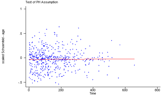
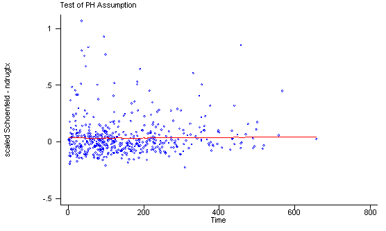
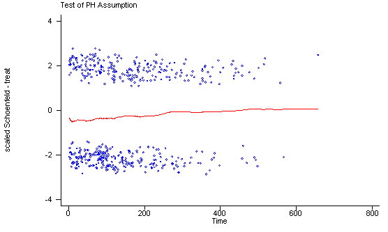
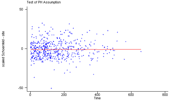
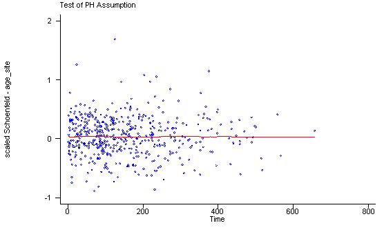
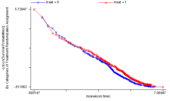
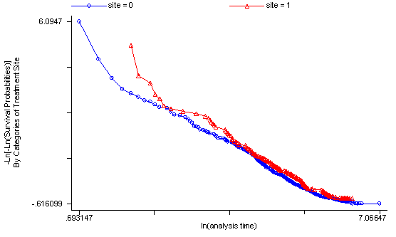
Another method of testing the proportionality assumption is by using the Schoenfeld and scaled Schoenfeld residuals which must first be saved through the stcox command. In the stphtest command we test the proportionality of the model as a whole and by using the detail option we get a test of proportionality for each predictor. By using the plot option we can also obtain a graph of the scaled Schoenfeld assumption. If the tests in the table are not significance (p-values over 0.05) then we can not reject proportionality and we assume that we do not have a violation of the proportional assumption. A horizontal line in the graphs is further indication that there is no violation of the proportionality assumption. The stphplot command uses log-log plots to test proportionality and if the lines in these plots are parallel then we have further indication that the predictors do not violate the proportionality assumption.
The predictor treat might warrant some closer examination since it does have a significant test and the curve in the graph is not completely horizontal. The graph from the stphplot command does not have completely parallel curves. However, we choose to leave treat in the model unaltered based on prior research.
quietly stcox age ndrugtx treat site c.age#i.site, schoenfeld(sch*) scaledsch(sca*)
stphtest, detail
stphtest, plot(age) msym(oh)
stphtest, plot(ndrugtx) msym(oh)
stphtest, plot(treat) msym(oh)
stphtest, plot(site) msym(oh)
stphtest, plot(c.age#1.site) msym(oh)

stphplot, by(treat) plot1(msym(oh)) plot2(msym(th))
stphplot, by(site) plot1(msym(oh)) plot2(msym(th))

drop sch1-sch5 sca1-sca5

Test of proportional hazards assumption

      Time:  Time
      ----------------------------------------------------------------
                  |       rho            chi2       df       Prob>chi2
      ------------+---------------------------------------------------
      age         |      0.01210         0.07        1         0.7912
      ndrugtx     |      0.05563         1.47        1         0.2260
      treat       |      0.10598         5.61        1         0.0179
      site        |      0.02336         0.25        1         0.6150
      age_site    |     -0.01350         0.08        1         0.7722
      ------------+---------------------------------------------------
      global test |                      8.27        5         0.1419
      ----------------------------------------------------------------
If one of the predictors were not proportional there are various solutions to consider. One solution is to include the time-dependent variable for the non-proportional predictors. Another solution is to stratify on the non-proportional predictor. The following is an example of stratification on the predictor treat. Note that treat is no longer included in the model statement instead it is specified in the strata statement.
stcox age ndrugtx site c.age#i.site, nohr strata(treat)


         failure _d:  censor
   analysis time _t:  time

Iteration 0:   log likelihood = -2525.8022
Iteration 1:   log likelihood =  -2511.524
Iteration 2:   log likelihood = -2510.8632
Iteration 3:   log likelihood = -2510.8606
Refining estimates:
Iteration 0:   log likelihood = -2510.8606

Stratified Cox regr. -- Breslow method for ties

No. of subjects =          610                  Number of obs    =         610
No. of failures =          495
Time at risk    =       142994
                                                LR chi2(4)       =       29.88
Log likelihood  =   -2510.8606                  Prob > chi2      =      0.0000

------------------------------------------------------------------------------
          _t |      Coef.   Std. Err.      z    P>|z|     [95% Conf. Interval]
-------------+----------------------------------------------------------------
         age |  -.0347463   .0092884    -3.74   0.000    -.0529512   -.0165413
     ndrugtx |   .0363728   .0076961     4.73   0.000     .0212888    .0514569
        site |  -1.251301   .5085532    -2.46   0.014    -2.248047   -.2545555
             |
  site#c.age |
          1  |   .0339858   .0155057     2.19   0.028     .0035951    .0643765
------------------------------------------------------------------------------
                                                           Stratified by treat
Graphing Survival Functions
Each covariate pattern will have a different survival function. The default survival function is for the covariate pattern where each predictor is set equal to zero. However, for many predictors this value is not meaningful because this value falls outside of the data such as age=0. It would be much more useful to specify an exact covariate pattern and generate a survival function for subjects with that specific covariate pattern.
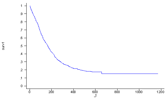
In the following example we want to graph the survival function for a subject who is 30 years old (age=30), has had 5 prior drug treatments (ndrugtx=5), and is currently getting the long treatment (treat=1) at site A (site=0 and agesite=30*0 = 0). We first output the baseline survival function for the covariate pattern where all predictors are set to zero. Then we raise the baseline survival function to the exponential to the linear combination of the coefficients and the values of the covariates in the covariate pattern of interest. Thus, in this particular instance the linear combination would be: -0.0336943*30+0.0364537*5 – 0.2674113*1 – 1.245928*0 – .0337728*0.
stcox age ndrugtx treat site c.age#i.site, nohr basesurv(surv0)
generate surv1 = surv0^exp( (-0.0336943*30+0.0364537*5 - 0.2674113))
line surv1 _t, sort ylab(0 .1 to 1) xlab(0 200 to 1200)
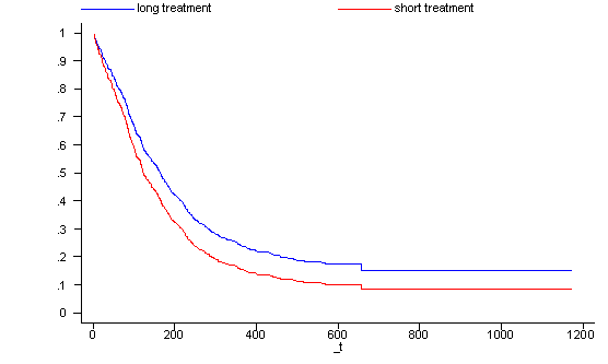
Looking at the survival function for one covariate pattern is sometimes not sufficient. It is often very useful to have a graph where we can compare the survival functions of different groups. In the following example we generate a graph with the survival functions for the two treatment groups where all the subjects are 30 years old (age=30), have had 5 prior drug treatments (ndrugtx=5) and are currently being treated at site A (site=0 and agesite=30*0=0). Thus, the two covariate patterns differ only in their values for treat.
generate surv2 = surv0^exp( (-0.0336943*30+0.0364537*5))
label variable surv1 "long treatment"
label variable surv2 "short treatment"
line surv1 surv2 _t, sort ylab(0 .1 to 1) xlab(0 200 to 1200)
drop surv0-surv2
Goodness of Fit of the Final Model
We can evaluate the fit of the model by using the Cox-Snell residuals. If the model fits the data well then the true cumulative hazard function conditional on the covariate vector has an exponential distribution with a hazard rate of one. This translates into fitting the model using the stcox command and specifying the mgale option which will generate the martingale residuals. Then we use the predict command with the csnell option to generate the Cox-Snell residuals for the model. We reset the data using the stset command specifying the variable cs, the variable containing the Cox-Snell residuals, as the time variable. We then use the sts generate command to create the Nelson-Aalen cumulative hazard function. Finally, we graph the Nelson-Aalen cumulative hazard function and the cs variable so that we can compare the hazard function to the diagonal line. If the hazard function follows the 45 degree line then we know that it approximately has an exponential distribution with a hazard rate of one and that the model fits the data well.
quietly stcox age ndrugtx treat site c.age#i.site, nohr mgale(mg)
predict cs, csnell

stset cs, failure(censor)
sts generate H = na
line H cs cs, sort xlab(0 1 to 4) ylab(0 1 to 4)
drop mg
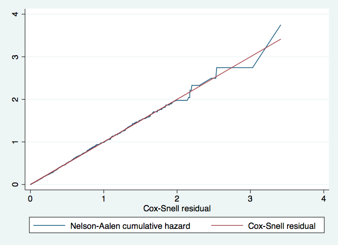
We see that the hazard function follows the 45 degree line very closely except for very large values of time. It is very common for models with censored data to have some wiggling at large values of time and it is not something which should cause much concern. Overall we would conclude that the final model fits the data very well.

