In the previous two chapters, we focused on issues regarding logistic regression analysis, such as how to create interaction variables and how to interpret the results of our logistic model. In order for our analysis to be valid, our model has to satisfy the assumptions of logistic regression. When the assumptions of logistic regression analysis are not met, we may have problems, such as biased coefficient estimates or very large standard errors for the logistic regression coefficients, and these problems may lead to invalid statistical inferences. Therefore, before we can use our model to make any statistical inference, we need to check that our model fits sufficiently well and check for influential observations that have impact on the estimates of the coefficients. In this chapter, we are going to focus on how to assess model fit, how to diagnose potential problems in our model and how to identify observations that have significant impact on model fit or parameter estimates. Let’s begin with a review of the assumptions of logistic regression.
- The true conditional probabilities are a logistic function of the independent variables.
- No important variables are omitted.
- No extraneous variables are included.
- The independent variables are measured without error.
- The observations are independent.
- The independent variables are not linear combinations of each other.
In this chapter, we are going to continue to use the apilog dataset.
use https://stats.idre.ucla.edu/stat/stata/webbooks/logistic/apilog, clear
3.1 Specification Error
When we build a logistic regression model, we assume that the logit of the outcome variable is a linear combination of the independent variables. This involves two aspects, as we are dealing with the two sides of our logistic regression equation. First, consider the link function of the outcome variable on the left hand side of the equation. We assume that the logit function (in logistic regression) is the correct function to use. Secondly, on the right hand side of the equation, we assume that we have included all the relevant variables, that we have not included any variables that should not be in the model, and the logit function is a linear combination of the predictors. It could happen that the logit function as the link function is not the correct choice or the relationship between the logit of outcome variable and the independent variables is not linear. In either case, we have a specification error. The misspecification of the link function is usually not too severe compared with using other alternative link function choices such as probit (based on the normal distribution). In practice, we are more concerned with whether our model has all the relevant predictors and if the linear combination of them is sufficient.
The Stata command linktest can be used to detect a specification error, and it is issued after the logit or logistic command. The idea behind linktest is that if the model is properly specified, one should not be able to find any additional predictors that are statistically significant except by chance. After the regression command (in our case, logit or logistic), linktest uses the predicted value (_hat) and predicted value squared (_hatsq) as the predictors to rebuild the model. The variable _hat should be a statistically significant predictor, since it is the predicted value from the model. This will be the case unless the model is completely misspecified. On the other hand, if our model is properly specified, variable _hatsq shouldn’t have much predictive power except by chance. Therefore, if _hatsq is significant, then the linktest is significant. This usually means that either we have omitted relevant variable(s) or our link function is not correctly specified.
Now let’s look at an example. In our api dataset, we have a variable called cred_ml, which is defined for 707 observations (schools) whose percentage of credential teachers are in the middle and lower range. For this subpopulation of schools, we believe that the variables yr_rnd, meals and cred_ml are powerful predictors for predicting if a school’s api score is high. So we ran the following logit command followed by the linktest command.
logit hiqual yr_rnd meals cred_ml, nolog          /*model 1*/

Logit estimates                                   Number of obs   =        707
                                                  LR chi2(3)      =     385.27
                                                  Prob > chi2     =     0.0000
Log likelihood = -156.38516                       Pseudo R2       =     0.5519

------------------------------------------------------------------------------
      hiqual |      Coef.   Std. Err.      z    P>|z|     [95% Conf. Interval]
-------------+----------------------------------------------------------------
      yr_rnd |  -1.185658     .50163    -2.36   0.018    -2.168835   -.2024813
       meals |  -.0932877   .0084252   -11.07   0.000    -.1098008   -.0767746
     cred_ml |   .7415145   .3152036     2.35   0.019     .1237268    1.359302
       _cons |   2.411226   .3987573     6.05   0.000     1.629676    3.192776

linktest, nolog


Logit estimates                                   Number of obs   =        707
                                                  LR chi2(2)      =     391.76
                                                  Prob > chi2     =     0.0000
Log likelihood = -153.13783                       Pseudo R2       =     0.5612

------------------------------------------------------------------------------
      hiqual |      Coef.   Std. Err.      z    P>|z|     [95% Conf. Interval]
-------------+----------------------------------------------------------------
        _hat |   1.209837   .1280197     9.45   0.000     .9589229    1.460751
      _hatsq |   .0735317    .026548     2.77   0.006     .0214986    .1255648
       _cons |  -.1381412   .1636431    -0.84   0.399    -.4588757    .1825933
------------------------------------------------------------------------------
We first see in the output from the logit command that the three predictors are all statistically significant predictors, and in the linktest that followed, the variable _hatsq is significant (with p-value = 0.006). This confirms, on one hand, that we have chosen meaningful predictors. On the other hand, it tells us that we have a specification error (since the linktest is significant). The first thing to do to remedy the situation is to see if we have included all of the relevant variables. More often than not, we thought we had included all of the variables, but we overlooked the possible interactions between the predictor variables. This may be the case with our model. So we try to add an interaction term to our model. We create an interaction variable ym=yr_rnd*meals and add it to our model and try the linktest again. First of all, the interaction term is significant with p-value =.015. Secondly, the linktest is no longer significant. This is an indication that that we should include the interaction term in the model, and by including it, we get a better model in terms of model specification.
gen ym=yr_rnd*meals
logit hiqual yr_rnd meals cred_ml ym , nolog /*model 2*/

Logit estimates                                   Number of obs   =        707
                                                  LR chi2(4)      =     390.13
                                                  Prob > chi2     =     0.0000
Log likelihood = -153.95333                       Pseudo R2       =     0.5589

------------------------------------------------------------------------------
      hiqual |      Coef.   Std. Err.      z    P>|z|     [95% Conf. Interval]
-------------+----------------------------------------------------------------
      yr_rnd |  -2.816989   .8625011    -3.27   0.001     -4.50746   -1.126518
       meals |  -.1014958   .0098204   -10.34   0.000    -.1207434   -.0822483
     cred_ml |   .7795476   .3205748     2.43   0.015     .1512326    1.407863
          ym |   .0459029   .0188068     2.44   0.015     .0090423    .0827635
       _cons |   2.668048    .429688     6.21   0.000     1.825875    3.510221
------------------------------------------------------------------------------

linktest

(Iterations omitted.)

Logit estimates                                   Number of obs   =        707
                                                  LR chi2(2)      =     390.87
                                                  Prob > chi2     =     0.0000
Log likelihood = -153.58393                       Pseudo R2       =     0.5600

------------------------------------------------------------------------------
      hiqual |      Coef.   Std. Err.      z    P>|z|     [95% Conf. Interval]
-------------+----------------------------------------------------------------
        _hat |   1.063142   .1154731     9.21   0.000     .8368188    1.289465
      _hatsq |   .0279257    .031847     0.88   0.381    -.0344934    .0903447
       _cons |  -.0605556   .1684181    -0.36   0.719    -.3906491    .2695378
------------------------------------------------------------------------------
Let’s now compare the two models we just built. From the output of our first logit command, we have the following regression equation:
logit(pred) = 2.411226 – 1.185658*yr_rnd -.0932877* meals + .7415145*cred_ml
This model does not have the interaction of the variables yr_rnd and meals. Therefore, the variable meals has the same predicting power regardless of whether a school is a year-around school or not. On the other hand, in the second model,
logit(pred) = 2.668048 – 2.816989*yr_rnd -.1014958* meals + .7795476*cred_ml + .0459029*ym,
since the interaction ym of yr_rnd and meals is included and is a significant predictor, the variable meals has different predicting power depending on if a school is a year-around school or not. More precisely, restricting our model to year-around schools (yr_rnd = 1), our second model becomes
logit(pred) = -.148941 -.05559291* meals + .7795476*cred_ml,
where the variable meals has only about half of the predicting power as in the first model (.05559291 versus .1014958). This makes sense since a year-around school usually has a higher percentage of students on free or reduced-priced meals than a non-year-around school. Therefore, within year-around schools, the variable meals is no longer as powerful as it is for a general school. This tells us that if we do not specify our model correctly, the effect of variable meals could be estimated with bias.
We need to keep in mind that linkest is simply a tool that assists in checking our models. It has its limits. It is better if we have a theory in mind to guide our model building, that we check our model against our theory, and that we validate our model based on our theory. Let’s look at another example where the linktest is not working so well. We use two binary variables, yr_rnd and cred_hl and one continuous variable meals as predictors for hiqual. The pseudo R-squared is .6286. But when we run linktest on this model, the _hatsq term is highly significant indicating a model specification error. Now if we take away the continuous variable and use the two binary variables in the model, the linktest is fine. But the pseudo R-squared is only .2023 now. Obviously, we can’t say that the smaller model is better model simply because the linktest does not provide evidence against it. What we can say is that both of the models have specification problems. But one specification problem can be detected by linktest and the other’s can’t.
logit hiqual yr_rnd cred_hl meals, nolog

Logistic regression                               Number of obs   =        875
                                                  LR chi2(3)      =     693.29
                                                  Prob > chi2     =     0.0000
Log likelihood = -204.84106                       Pseudo R2       =     0.6286

------------------------------------------------------------------------------
      hiqual |      Coef.   Std. Err.      z    P>|z|     [95% Conf. Interval]
-------------+----------------------------------------------------------------
      yr_rnd |  -.3937266   .4404698    -0.89   0.371    -1.257031    .4695783
     cred_hl |   .9656431    .311385     3.10   0.002     .3553396    1.575947
       meals |  -.1057442    .007864   -13.45   0.000    -.1211572   -.0903311
       _cons |   2.752695   .3837638     7.17   0.000     2.000531    3.504858
------------------------------------------------------------------------------

linktest, nolog

Logistic regression                               Number of obs   =        875
                                                  LR chi2(2)      =     706.58
                                                  Prob > chi2     =     0.0000
Log likelihood = -198.19639                       Pseudo R2       =     0.6406

------------------------------------------------------------------------------
      hiqual |      Coef.   Std. Err.      z    P>|z|     [95% Conf. Interval]
-------------+----------------------------------------------------------------
        _hat |   1.149581   .0894218    12.86   0.000     .9743173    1.324844
      _hatsq |   .0744209   .0184489     4.03   0.000     .0382617    .1105802
       _cons |  -.2430064   .1468835    -1.65   0.098    -.5308928      .04488
------------------------------------------------------------------------------

logit hiqual yr_rnd cred_hl, nolog

Logistic regression                               Number of obs   =        875
                                                  LR chi2(2)      =     223.09
                                                  Prob > chi2     =     0.0000
Log likelihood = -439.93663                       Pseudo R2       =     0.2023

------------------------------------------------------------------------------
      hiqual |      Coef.   Std. Err.      z    P>|z|     [95% Conf. Interval]
-------------+----------------------------------------------------------------
      yr_rnd |  -1.167753   .2949081    -3.96   0.000    -1.745763    -.589744
     cred_hl |    2.32597   .2104116    11.05   0.000     1.913571    2.738369
       _cons |  -2.173594   .1929948   -11.26   0.000    -2.551857   -1.795331
------------------------------------------------------------------------------

linktest, nolog

Logistic regression                               Number of obs   =        875
                                                  LR chi2(2)      =     223.10
                                                  Prob > chi2     =     0.0000
Log likelihood =  -439.9364                       Pseudo R2       =     0.2023

------------------------------------------------------------------------------
      hiqual |      Coef.   Std. Err.      z    P>|z|     [95% Conf. Interval]
-------------+----------------------------------------------------------------
        _hat |   .9941096   .2856893     3.48   0.001     .4341687     1.55405
      _hatsq |  -.0025741   .1195847    -0.02   0.983    -.2369558    .2318077
       _cons |   .0006538   .0932373     0.01   0.994     -.182088    .1833956
------------------------------------------------------------------------------
We have seen earlier that lacking an interaction term could cause a model specification problem. Similarly, we could also have a model specification problem if some of the predictor variables are not properly transformed. For example, the change of a dependent variable with respect to a predictor may not be linear, but only the linear term is used as a predictor in the model. To address this, a Stata program called boxtid can be used. It is a user-written program that you can download over the internet and use (type “search boxtid“). boxtid stands for Box-Tidwell model, which transforms a predictor using power transformations and finds the best power for model fit based on maximal likelihood estimate. More precisely, a predictor x is transformed into B1 + B2xp and the best p is found using maximal likelihood estimate. Besides estimating the power transformation, boxtid also estimates exponential transformations, which can be viewed as power functions on the exponential scale.
Let’s look at another model where we predict hiqaul from yr_rnd and meals. We’ll start with a model with only two predictors. The linktest is significant, indicating problem with model specification. We then use boxtid, and it displays the best transformation of the predictor variables, if needed.
logit ogit hiqual yr_rnd meals , nologLogistic regression Number of obs = 1200 LR chi2(2) = 898.30 Prob > chi2 = 0.0000 Log likelihood = -308.27755 Pseudo R2 = 0.5930------------------------------------------------------------------------------ hiqual | Coef. Std. Err. z P>|z| [95% Conf. Interval] -------------+---------------------------------------------------------------- yr_rnd | -.9908119 .3545667 -2.79 0.005 -1.68575 -.2958739 meals | -.1074156 .0064857 -16.56 0.000 -.1201274 -.0947039 _cons | 3.61557 .2418967 14.95 0.000 3.141462 4.089679 ------------------------------------------------------------------------------linktest, nologLogistic regression Number of obs = 1200 LR chi2(2) = 908.87 Prob > chi2 = 0.0000 Log likelihood = -302.99327 Pseudo R2 = 0.6000------------------------------------------------------------------------------ hiqual | Coef. Std. Err. z P>|z| [95% Conf. Interval] -------------+---------------------------------------------------------------- _hat | 1.10755 .0724056 15.30 0.000 .9656379 1.249463 _hatsq | .0622644 .0174384 3.57 0.000 .0280858 .096443 _cons | -.1841694 .1185283 -1.55 0.120 -.4164805 .0481418 ------------------------------------------------------------------------------boxtid logit hiqual yr_rnd mealsIteration 0: Deviance = 608.6424 Iteration 1: Deviance = 608.6373 (change = -.0050887) Iteration 2: Deviance = 608.6373 (change = -.0000592) -> gen double Imeal__1 = X^0.5535-.7047873475 if e(sample) -> gen double Imeal__2 = X^0.5535*ln(X)+.4454623098 if e(sample) (where: X = (meals+1)/100)[Total iterations: 2]Box-Tidwell regression modelLogistic regression Number of obs = 1200 LR chi2(3) = 906.22 Prob > chi2 = 0.0000 Log likelihood = -304.31863 Pseudo R2 = 0.5982------------------------------------------------------------------------------ hiqual | Coef. Std. Err. z P>|z| [95% Conf. Interval] -------------+---------------------------------------------------------------- Imeal__1 | -12.13661 1.60761 -7.55 0.000 -15.28747 -8.985755 Imeal_p1 | .0016505 1.961413 0.00 0.999 -3.842647 3.845948 yr_rnd | -.998601 .3598947 -2.77 0.006 -1.703982 -.2932205 _cons | -1.9892 .1502115 -13.24 0.000 -2.283609 -1.694791 ------------------------------------------------------------------------------ meals | -.1074156 .0064857 -16.562 Nonlin. dev. 7.918 (P = 0.005) p1 | .5535294 .1622327 3.412 ------------------------------------------------------------------------------ Deviance: 608.637.
The variable meals is statistically significant with p-value =.005 for being a nonlinear term. The variable yr_rnd as a binary variable does not have a nonlinear form. The null hypothesis is that the predictor variable meals is of a linear term, or, equivalently, p1 = 1. But it shows that p1 is around .55 to be optimal. (Look closer at the output following the last iteration.) This suggests a square-root transformation of the variable meals. So let’s try this approach and replace the variable meals with the square-root of itself.
gen m2=meals^.5
logit hiqual yr_rnd m2, nolog
Logistic regression Number of obs = 1200 LR chi2(2) = 905.87 Prob > chi2 = 0.0000 Log likelihood = -304.48899 Pseudo R2 = 0.5980------------------------------------------------------------------------------ hiqual | Coef. Std. Err. z P>|z| [95% Conf. Interval] -------------+---------------------------------------------------------------- yr_rnd | -1.000602 .3601437 -2.78 0.005 -1.70647 -.2947332 m2 | -1.245371 .0742987 -16.76 0.000 -1.390994 -1.099749 _cons | 7.008795 .4495493 15.59 0.000 6.127694 7.889895 ------------------------------------------------------------------------------linktest, nolog Logistic regression Number of obs = 1200 LR chi2(2) = 905.91 Prob > chi2 = 0.0000 Log likelihood = -304.47104 Pseudo R2 = 0.5980------------------------------------------------------------------------------ hiqual | Coef. Std. Err. z P>|z| [95% Conf. Interval] -------------+---------------------------------------------------------------- _hat | .9957904 .0629543 15.82 0.000 .8724022 1.119179 _hatsq | -.0042551 .0224321 -0.19 0.850 -.0482211 .0397109 _cons | .0120893 .1237232 0.10 0.922 -.2304036 .2545823 ------------------------------------------------------------------------------
This shows that sometimes the logit of the outcome variable may not be a linear combination of the predictors variables, but a linear combination of transformed predictor variables as well as the interaction terms as we have shown previously.
We have only scratched the surface on how to deal with the issue of specification errors. In practice, a combination of a good grasp of the theory behind the model and a bundle of statistical tools to detect specification error and other potential problems is necessary to guide us through model building. For more detailed discussion and examples, see John Fox’s Regression Diagnostics and Menard’s Applied Logistic Regression Analysis.
3.2 Goodness-of-fit
We have seen from our previous lessons that Stata’s output of logistic regression contains the log likelihood chi-square and pseudo R-square for the model. These measures, together with others that we are also going to discuss in this section, give us a general gauge on how the model fits the data. Let’s start with a model that we have shown previously.
use https://stats.idre.ucla.edu/stat/Stata/webbooks/logistic/apilog, clear
gen ym=yr_rnd*meals
logit hiqual yr_rnd meals cred_ml ym
Iteration 0: log likelihood = -349.01971 Iteration 1: log likelihood = -192.43886 Iteration 2: log likelihood = -160.94663 Iteration 3: log likelihood = -154.63544 Iteration 4: log likelihood = -153.96521 Iteration 5: log likelihood = -153.95333 Iteration 6: log likelihood = -153.95333Logistic regression Number of obs = 707 LR chi2(4) = 390.13 Prob > chi2 = 0.0000 Log likelihood = -153.95333 Pseudo R2 = 0.5589 ------------------------------------------------------------------------------ hiqual | Coef. Std. Err. z P>|z| [95% Conf. Interval] -------------+---------------------------------------------------------------- yr_rnd | -2.816989 .8625011 -3.27 0.001 -4.50746 -1.126518 meals | -.1014958 .0098204 -10.34 0.000 -.1207434 -.0822483 cred_ml | .7795476 .3205748 2.43 0.015 .1512326 1.407863 ym | .0459029 .0188068 2.44 0.015 .0090423 .0827635 _cons | 2.668048 .429688 6.21 0.000 1.825875 3.510221 ------------------------------------------------------------------------------
The log likelihood chi-square is an omnibus test to see if the model as a whole is statistically significant. It is 2 times the difference between the log likelihood of the current model and the log likelihood of the intercept-only model. Since Stata always starts its iteration process with the intercept-only model, the log likelihood at Iteration 0 shown above corresponds to the log likelihood of the empty model. The four degrees of freedom comes from the four predictor variables that the current model has.
di 2*(349.01917-153.95333)
390.13168
A pseudo R-square is in slightly different flavor, but captures more or less the same thing in that it is the proportion of change in terms of likelihood.
 di (349.01971-153.95333)/349.01971
.55889789
It is a “pseudo” R-square because it is unlike the R-square found in OLS regression, where R-square measures the proportion of variance explained by the model. The pseudo R-square is not measured in terms of variance, since in logistic regression the variance is fixed as the variance of the standard logistic distribution. It is a proportion in terms of the log likelihood.
Another commonly used test of model fit is the Hosmer and Lemeshow’s goodness-of-fit test. The idea behind the Hosmer and Lemeshow’s goodness-of-fit test is that the predicted frequency and observed frequency should match closely, and that the more closely they match, the better the fit. The Hosmer-Lemeshow goodness-of-fit statistic is computed as the Pearson chi-square from the contingency table of observed frequencies and expected frequencies. Similar to a test of association of a two-way table, a good fit as measured by Hosmer and Lemeshow’s test will yield a large p-value. When there are continuous predictors in the model, there will be many cells defined by the predictor variables, making a very large contingency table, which would yield significant result more than often. So a common practice is to combine the patterns formed by the predictor variables into 10 groups and form a contingency table of 2 by 10.
lfit, group(10) tableLogistic model for hiqual, goodness-of-fit test(Table collapsed on quantiles of estimated probabilities) +--------------------------------------------------------+ | Group | Prob | Obs_1 | Exp_1 | Obs_0 | Exp_0 | Total | |-------+--------+-------+-------+-------+-------+-------| | 1 | 0.0016 | 0 | 0.1 | 71 | 70.9 | 71 | | 2 | 0.0033 | 1 | 0.2 | 73 | 73.8 | 74 | | 3 | 0.0054 | 0 | 0.3 | 74 | 73.7 | 74 | | 4 | 0.0096 | 1 | 0.5 | 64 | 64.5 | 65 | | 5 | 0.0206 | 1 | 1.0 | 69 | 69.0 | 70 | |-------+--------+-------+-------+-------+-------+-------| | 6 | 0.0623 | 4 | 2.5 | 69 | 70.5 | 73 | | 7 | 0.1421 | 2 | 6.6 | 66 | 61.4 | 68 | | 8 | 0.4738 | 24 | 22.0 | 50 | 52.0 | 74 | | 9 | 0.7711 | 44 | 43.3 | 25 | 25.7 | 69 | | 10 | 0.9692 | 61 | 61.6 | 8 | 7.4 | 69 | +--------------------------------------------------------+number of observations = 707 number of groups = 10 Hosmer-Lemeshow chi2(8) = 9.15 Prob > chi2 = 0.3296
With a p-value of .33, we can say that Hosmer and Lemeshow’s goodness-of-fit test indicates that our model fits the data well.
There are many other measures of model fit, such AIC (Akaike Information Criterion) and BIC (Bayesian Information Criterion). A command called fitstat will display most of them after a model.
fitstatMeasures of Fit for logit of hiqualLog-Lik Intercept Only: -349.020 Log-Lik Full Model: -153.953 D(702): 307.907 LR(4): 390.133 Prob > LR: 0.000 McFadden's R2: 0.559 McFadden's Adj R2: 0.545 Maximum Likelihood R2: 0.424 Cragg & Uhler's R2: 0.676 McKelvey and Zavoina's R2: 0.715 Efron's R2: 0.585 Variance of y*: 11.546 Variance of error: 3.290 Count R2: 0.904 Adj Count R2: 0.507 AIC: 0.450 AIC*n: 317.907 BIC: -4297.937 BIC': -363.889
Many times, fitstat is used to compare models. Let’s say we want to compare the current model which includes the interaction term of yr_rnd and meals with a model without the interaction term. We can use the fitsat options using and saving to compare models.
logit

Logistic regression                               Number of obs   =        707
                                                  LR chi2(4)      =     390.13
                                                  Prob > chi2     =     0.0000
Log likelihood = -153.95333                       Pseudo R2       =     0.5589
------------------------------------------------------------------------------ hiqual | Coef. Std. Err. z P>|z| [95% Conf. Interval] -------------+---------------------------------------------------------------- yr_rnd | -2.816989 .8625011 -3.27 0.001 -4.50746 -1.126518 meals | -.1014958 .0098204 -10.34 0.000 -.1207434 -.0822483 cred_ml | .7795476 .3205748 2.43 0.015 .1512326 1.407863 ym | .0459029 .0188068 2.44 0.015 .0090423 .0827635 _cons | 2.668048 .429688 6.21 0.000 1.825875 3.510221 ------------------------------------------------------------------------------fitstat, saving(m1)Measures of Fit for logit of hiqualLog-Lik Intercept Only: -349.020 Log-Lik Full Model: -153.953 D(702): 307.907 LR(4): 390.133 Prob > LR: 0.000 McFadden's R2: 0.559 McFadden's Adj R2: 0.545 Maximum Likelihood R2: 0.424 Cragg & Uhler's R2: 0.676 McKelvey and Zavoina's R2: 0.715 Efron's R2: 0.585 Variance of y*: 11.546 Variance of error: 3.290 Count R2: 0.904 Adj Count R2: 0.507 AIC: 0.450 AIC*n: 317.907 BIC: -4297.937 BIC': -363.889(Indices saved in matrix fs_m1)logit hiqual yr_rnd meals cred_ml, nologLogistic regression Number of obs = 707 LR chi2(3) = 385.27 Prob > chi2 = 0.0000 Log likelihood = -156.38516 Pseudo R2 = 0.5519------------------------------------------------------------------------------ hiqual | Coef. Std. Err. z P>|z| [95% Conf. Interval] -------------+---------------------------------------------------------------- yr_rnd | -1.185658 .50163 -2.36 0.018 -2.168835 -.2024813 meals | -.0932877 .0084252 -11.07 0.000 -.1098008 -.0767746 cred_ml | .7415145 .3152036 2.35 0.019 .1237268 1.359302 _cons | 2.411226 .3987573 6.05 0.000 1.629676 3.192776 ------------------------------------------------------------------------------fitstat, using(m1)Measures of Fit for logit of hiqualCurrent Saved Difference Model: logit logit N: 707 707 0 Log-Lik In,t Only: -349.020 -349.020 0.000 Log-Lik Full Model: -156.385 -153.953 -2.432 D: 312.770(703) 307.907(702) 4.864(1) LR: 385.269(3) 390.133(4) 4.864(1) Prob > LR: 0.000 0.000 0.027 McFadden's R2: 0.552 0.559 -0.007 McFadden's Adj R2: 0.540 0.545 -0.004 Maximum Likelihood R2: 0.420 0.424 -0.004 Cragg & Uhler's R2: 0.670 0.676 -0.006 McKelvey and Zavoina's R2: 0.742 0.715 0.027 Efron's R2: 0.587 0.585 0.002 Variance of y*: 12.753 11.546 1.207 Variance of error: 3.290 3.290 0.000 Count R2: 0.909 0.904 0.006 Adj Count R2: 0.536 0.507 0.029 AIC: 0.454 0.450 0.004 AIC*n: 320.770 317.907 2.864 BIC: -4299.634 -4297.937 -1.697 BIC': -365.586 -363.889 -1.697Difference of 1.697 in BIC' provides weak support for current model.Note: p-value for difference in LR is only valid if models are nested.
The first fitstat displays and saves the fit statistics for the larger model, and the second one uses the saved information to compare with the current model. The result supports the model with no interaction over the model with the interaction, but only weakly. On the other hand, we have already shown that the interaction term is significant. But if we look more closely, we can see its coefficient is fairly small in the logit scale and is very close to 1 in the odds ratio scale. So the substantive meaning of the interaction being statistically significant may not be as prominent as it looks.
As we can see from the fitstat command that there are many different versions of pseudo R-squares displayed. One of them is the McFadden’s R-square reported by the logit command as the Pseudo R-square. As mentioned in Hosmer and Lemeshow’s Applied Logistic Regression, all the various pseudo R-squares are low when compared to R-square values for a good linear model. So even though they may be helpful in the modeling process, they are not recommended to be routinely published. ( see page 167.) Our pseudo R-square of .59 is fairly high. Commonly we see them around .2 and .4 range.
3.3 Multicollinearity
Multicollinearity (or collinearity for short) occurs when two or more independent variables in the model are approximately determined by a linear combination of other independent variables in the model. The degree of multicollinearity can vary and can have different effects on the model. When perfect collinearity occurs, that is, when one independent variable is a perfect linear combination of the others, it is impossible to obtain a unique estimate of regression coefficients with all the independent variables in the model. What Stata does in this case is to drop a variable that is a perfect linear combination of the others, leaving only the variables that are not exactly linear combinations of others in the model to assure unique estimate of regression coefficients. For example, we can artificially create a new variable called perli as the sum of yr_rnd and meals. Notice that the only purpose of this example and the creation of the variable perli is to show what Stata does when perfect collinearity occurs. Notice that Stata issues a note, informing us that the variable yr_rnd has been dropped from the model due to collinearity. We cannot assume that the variable that Stata drops from the model is the “correct” variable to omit from the model; rather, we need to rely on theory to determine which variable should be omitted.
use https://stats.idre.ucla.edu/stat/Stata/webbooks/logistic/apilog, clear
gen perli=yr_rnd+meals
logit hiqual perli meals yr_rnd


note: yr_rnd dropped due to collinearity
(Iterations omitted.)

Logit estimates                                   Number of obs   =       1200
                                                  LR chi2(2)      =     898.30
                                                  Prob > chi2     =     0.0000
Log likelihood = -308.27755                       Pseudo R2       =     0.5930

------------------------------------------------------------------------------
      hiqual |      Coef.   Std. Err.      z    P>|z|     [95% Conf. Interval]
-------------+----------------------------------------------------------------
       perli |  -.9908119   .3545667    -2.79   0.005     -1.68575   -.2958739
       meals |   .8833963   .3542845     2.49   0.013     .1890113    1.577781
       _cons |    3.61557   .2418967    14.95   0.000     3.141462    4.089679
------------------------------------------------------------------------------
Moderate multicollinearity is fairly common since any correlation among the independent variables is an indication of collinearity. But when severe multicollinearity occurs, the standard errors for the coefficients tend to be very large (inflated), and sometimes the estimated logistic regression coefficients can be highly unreliable. Let’s consider the following example. In this model, the dependent variable will be hiqual, and the predictor variables will include avg_ed, yr_rnd, meals, full, and the interaction between yr_rnd and full, yxfull. After the logit procedure, we will also run a goodness-of-fit test. Notice that the goodness-of-fit test indicates that, overall, our model fits pretty well.
gen yxfull=  yr_rnd*full
logit  hiqual avg_ed yr_rnd meals full yxfull, nolog or

Logit estimates                                   Number of obs   =       1158
                                                  LR chi2(5)      =     933.71
                                                  Prob > chi2     =     0.0000
Log likelihood = -263.83452                       Pseudo R2       =     0.6389

------------------------------------------------------------------------------
      hiqual | Odds Ratio   Std. Err.      z    P>|z|     [95% Conf. Interval]
-------------+----------------------------------------------------------------
      avg_ed |   7.163138   2.041592     6.91   0.000     4.097315    12.52297
      yr_rnd |   70719.31     208020     3.80   0.000     221.6864    2.26e+07
       meals |   .9240607   .0073503    -9.93   0.000     .9097661      .93858
        full |   1.051269   .0152644     3.44   0.001     1.021773    1.081617
      yxfull |   .8755202   .0284632    -4.09   0.000     .8214734    .9331228
------------------------------------------------------------------------------
lfit, group(10)Logistic model for hiqual, goodness-of-fit test(Table collapsed on quantiles of estimated probabilities)number of observations = 1158 number of groups = 10 Hosmer-Lemeshow chi2(8) = 5.50 Prob > chi2 = 0.7034
Nevertheless, notice the odd ratio and standard error for the variable yr_rnd are incredibly high. Apparently something went wrong. A direct cause for the incredibly large odd ratio and very large standard error is the multicollinearity among the independent variables. We can use a program called collin to detect the multicollinearity. You can download the program from the ATS website of Stata programs for teaching and research. (or use “search collin” and then follow the link to it.)
collin avg_ed yr_rnd meals full yxfull

  Collinearity Diagnostics

                        SQRT                           Cond
  Variable       VIF    VIF    Tolerance  Eigenval     Index
-------------------------------------------------------------
    avg_ed      3.28    1.81    0.3050     2.7056     1.0000
    yr_rnd     35.53    5.96    0.0281     1.4668     1.3581
     meals      3.80    1.95    0.2629     0.6579     2.0279
      full      1.72    1.31    0.5819     0.1554     4.1728
    yxfull     34.34    5.86    0.0291     0.0144    13.7284
-------------------------------------------------------------
  Mean VIF     15.73              Condition Number   13.7284
All the measures in the above output are measures of the strength of the interrelationships among the variables. Two commonly used measures are tolerance (an indicator of how much collinearity that a regression analysis can tolerate) and VIF (variance inflation factor-an indicator of how much of the inflation of the standard error could be caused by collinearity). The tolerance for a particular variable is 1 minus the R2 that results from the regression of the other variables on that variable. The corresponding VIF is simply 1/tolerance. If all of the variables are orthogonal to each other, in other words, completely uncorrelated with each other, both the tolerance and VIF are 1. If a variable is very closely related to another variable(s), the tolerance goes to 0, and the variance inflation gets very large. For example, in the output above, we see that the tolerance and VIF for the variable yxfull is 0.0291 and 34.34, respectively. We can reproduce these results by doing the corresponding regression.
regress  yxfull full meals yr_rnd avg_ed

      Source |       SS       df       MS              Number of obs =    1158
-------------+------------------------------           F(  4,  1153) = 9609.80
       Model |  1128915.43     4  282228.856           Prob > F      =  0.0000
    Residual |  33862.2808  1153  29.3688472           R-squared     =  0.9709
-------------+------------------------------           Adj R-squared =  0.9708
       Total |  1162777.71  1157   1004.9937           Root MSE      =  5.4193

------------------------------------------------------------------------------
      yxfull |      Coef.   Std. Err.      t    P>|t|     [95% Conf. Interval]
-------------+----------------------------------------------------------------
        full |   .2313279   .0140312    16.49   0.000     .2037983    .2588574
       meals |    -.00088   .0099863    -0.09   0.930    -.0204733    .0187134
      yr_rnd |   83.10644   .4408941   188.50   0.000      82.2414    83.97149
      avg_ed |  -.4611434   .3744277    -1.23   0.218    -1.195779    .2734925
       _cons |  -19.38205   2.100101    -9.23   0.000     -23.5025    -15.2616
------------------------------------------------------------------------------
Notice that the R2 is .9709. Therefore, the tolerance is 1-.9709 = .0291. The VIF is 1/.0291 = 34.36 (the difference between 34.34 and 34.36 being rounding error). As a rule of thumb, a tolerance of 0.1 or less (equivalently VIF of 10 or greater) is a cause for concern.
Now we have seen what tolerance and VIF measure and we have been convinced that there is a serious collinearity problem, what do we do about it? Notice that in the above regression, the variables full and yr_rnd are the only significant predictors and the coefficient for yr_rnd is very large. This is because often times when we create an interaction term, we also create some collinearity problem. This can be seen in the output of the correlation below. One way of fixing the collinearity problem is to center the variable full as shown below. We use the sum command to obtain the mean of the variable full, and then generate a new variable called fullc, which is full minus its mean. Next, we generate the interaction of yr_rnd and fullc, called yxfc. Finally, we run the logit command with fullc and yxfc as predictors instead of full and yxfull. Remember that if you use a centered variable as a predictor, you should create any necessary interaction terms using the centered version of that variable (rather than the uncentered version).
corr yxfull yr_rnd full
(obs=1200)

             |   yxfull   yr_rnd     full
-------------+---------------------------
      yxfull |   1.0000
      yr_rnd |   0.9810   1.0000
        full |  -0.1449  -0.2387   1.0000

sum full

    Variable |     Obs        Mean   Std. Dev.       Min        Max
-------------+-----------------------------------------------------
        full |    1200    88.12417   13.39733         13        100

gen fullc=full-r(mean)
gen yxfc=yr_rnd*fullc
corr yxfc  yr_rnd fullc
(obs=1200)

             |     yxfc   yr_rnd    fullc
-------------+---------------------------
        yxfc |   1.0000
      yr_rnd |  -0.3910   1.0000
       fullc |   0.5174  -0.2387   1.0000


logit  hiqual avg_ed yr_rnd meals fullc yxfc, nolog or

Logit estimates                                   Number of obs   =       1158
                                                  LR chi2(5)      =     933.71
                                                  Prob > chi2     =     0.0000
Log likelihood = -263.83452                       Pseudo R2       =     0.6389

------------------------------------------------------------------------------
      hiqual | Odds Ratio   Std. Err.      z    P>|z|     [95% Conf. Interval]
-------------+----------------------------------------------------------------
      avg_ed |   7.163138   2.041592     6.91   0.000     4.097315    12.52297
      yr_rnd |   .5778193   .2126551    -1.49   0.136      .280882    1.188667
       meals |   .9240607   .0073503    -9.93   0.000     .9097661      .93858
       fullc |   1.051269   .0152644     3.44   0.001     1.021773    1.081617
        yxfc |   .8755202   .0284632    -4.09   0.000     .8214734    .9331228
------------------------------------------------------------------------------

collin hiqual avg_ed yr_rnd meals fullc yxfc

  Collinearity Diagnostics

                        SQRT                           Cond
  Variable       VIF    VIF    Tolerance  Eigenval     Index
-------------------------------------------------------------
    hiqual      2.40    1.55    0.4173     3.1467     1.0000
    avg_ed      3.46    1.86    0.2892     1.2161     1.6086
    yr_rnd      1.24    1.12    0.8032     0.7789     2.0100
     meals      4.46    2.11    0.2241     0.4032     2.7938
     fullc      1.72    1.31    0.5816     0.3044     3.2153
      yxfc      1.54    1.24    0.6488     0.1508     4.5685
-------------------------------------------------------------
  Mean VIF      2.47              Condition Number    4.5685
We display the correlation matrix using the corr command before and after the centering and notice how much change the centering has produced. The centering of the variable full in this case has fixed the problem of collinearity, and our model fits well overall. The variable yr_rnd is no longer a significant predictor, but the interaction term between yr_rnd and full is. By being able to keep all the predictors in our model, it will be easy for us to interpret the effect of each of the predictors. This centering method can be considered as a special case of a transformation of the variables. Transformation of the variables is the best remedy for multicollinearity when it works, since we don’t lose any variables from our model. But the choice of transformation is often difficult to make, other than the straightforward ones such as centering. Other commonly used transformation include log-transformation and square-transformation. Other commonly suggested remedies include deleting some of the variables and increasing sample size to get more information. The first one is not always a good option, as it might lead to a misspecified model, and the second option is not always possible. We refer our readers to Berry and Feldman’s Multiple Regression in Practice (1985, pp. 46-50) for more detailed discussion of remedies for collinearity.
3.4 Influential Observations
So far, we have seen how to detect potential problems in model building. We will focus now on detecting potential observations that have a significant impact on the model. There are several reasons that we need to detect influential observations. First, these might be data entry errors. Secondly, influential observations may be of interest by themselves for us to study. Also, influential data points may yield biased regression coefficient estimates. In OLS regression, we have several types of residuals and influence measures that help us understand how each observation behaves in the model, such as if the observation is too far away from the rest of the observations, or if the observation has too much leverage on the regression line. Similar techniques have been developed for logistic regression as well.
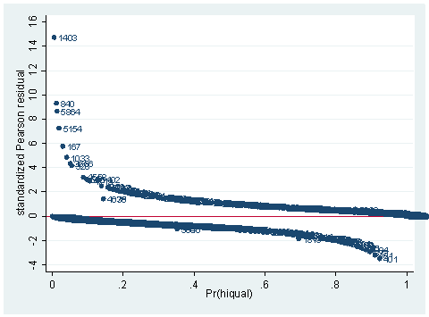
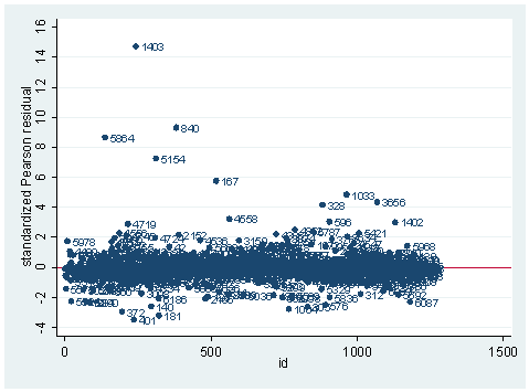
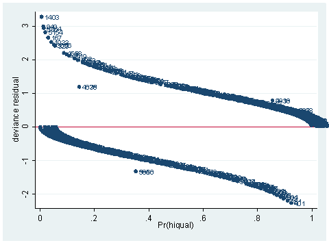
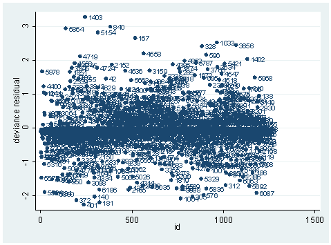
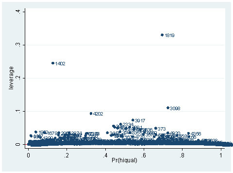
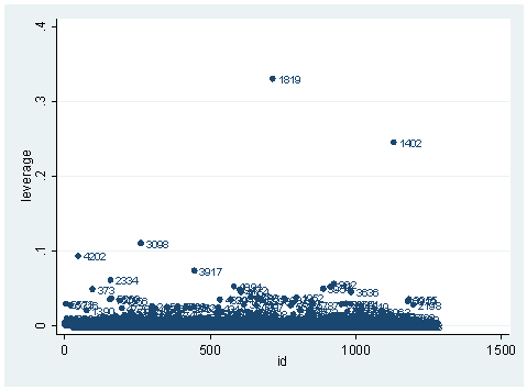
Pearson residuals and its standardized version is one type of residual measures. Pearson residuals are defined to be the standardized difference between the observed frequency and the predicted frequency. They measure the relative deviations between the observed and fitted values. Deviance residual is another type of residual measures. It measures the disagreement between the maxima of the observed and the fitted log likelihood functions. Since logistic regression uses the maximal likelihood principle, the goal in logistic regression is to minimize the sum of the deviance residuals. Therefore, this residual is parallel to the raw residual in OLS regression, where the goal is to minimize the sum of squared residuals. Another statistic, sometimes called the hat diagonal since technically it is the diagonal of the hat matrix, measures the leverage of an observation. It is also sometimes called the Pregibon leverage. These three statistics, Pearson residual, deviance residual and Pregibon leverage are considered to be the three basic building blocks for logistic regression diagnostics. They can be obtained from Stata after the logit or logistic command. A good way of looking at them is to graph them against either the predicted probabilities or simply case numbers. Let us see them in an example. We continue to use the model built in our last section, as shown below. We’ll get both the standardized Pearson residuals, deviance residuals and the leverage (hat diagonal) and plot them against the predicted probabilities and index numbers.
use https://stats.idre.ucla.edu/stat/Stata/webbooks/logistic/apilog, clear
sum full
gen fullc=full-r(mean)
gen yxfc=yr_rnd*fullc
logit  hiqual avg_ed yr_rnd meals fullc yxfc, nolog

Logistic regression                               Number of obs   =       1158
                                                  LR chi2(5)      =     933.71
                                                  Prob > chi2     =     0.0000
Log likelihood = -263.83452                       Pseudo R2       =     0.6389
------------------------------------------------------------------------------ hiqual | Coef. Std. Err. z P>|z| [95% Conf. Interval] -------------+---------------------------------------------------------------- avg_ed | 1.968948 .2850136 6.91 0.000 1.410332 2.527564 yr_rnd | -.5484941 .3680305 -1.49 0.136 -1.269821 .1728325 meals | -.0789775 .0079544 -9.93 0.000 -.0945677 -.0633872 fullc | .0499983 .01452 3.44 0.001 .0215397 .0784569 yxfc | -.1329371 .0325101 -4.09 0.000 -.1966557 -.0692185 _cons | -3.655163 1.016972 -3.59 0.000 -5.648392 -1.661935 ------------------------------------------------------------------------------predict p predict stdres, rstandscatter stdres p, mlabel(snum) ylab(-4(2) 16) yline(0)
gen id=_n scatter stdres id, mlab(snum) ylab(-4(2) 16) yline(0)
predict dv, dev scatter dv p, mlab(snum) yline(0)
scatter dv id, mlab(snum)
predict hat, hat scatter hat p, mlab(snum) yline(0)
scatter hat id, mlab(snum)
As you can see, we have produced two types of plots using these statistics: the plots of the statistics against the predicted values, and the plots of these statistics against the index id (it is therefore also called an index plot.) These two types of plots basically convey the same information. The data points seem to be more spread out on index plots, making it easier to see the index for the extreme observations. What do we see from these plots? We see some observations that are far away from most of the other observations. These are the points that need particular attention. For example, the observation with school number 1403 has a very high Pearson and deviance residual. The observed outcome hiqual is 1 but the predicted probability is very, very low. This leads to large residuals. But notice that observation 1403 is not that bad in terms of leverage. That is to say, that by not including this particular observation, our logistic regression estimate won’t be too much different from the model that includes this observation. Let’s list the most outstanding observations based on the graphs.
clist if snum==1819 | snum==1402 | snum==1403
Observation 243
snum 1403 dnum 315 schqual high hiqual high
yr_rnd yrrnd meals 100 enroll 497 cred low
cred_ml low cred_hl low pared medium pared_ml medium
pared_hl . api00 808 api99 824 full 59
some_col 28 awards No ell 27 avg_ed 2.19
fullc -29.12417 yxfc -29.12417 stdres 14.71427 p .0046147
id 243 dv 3.27979 hat .0037408
Observation 715
snum 1819 dnum 401 schqual low hiqual not high
yr_rnd yrrnd meals 100 enroll 872 cred low
cred_ml low cred_hl low pared low pared_ml low
pared_hl low api00 406 api99 372 full 51
some_col 0 awards Yes ell 74 avg_ed 5
fullc -37.12417 yxfc -37.12417 stdres -1.844296 p .6947385
id 715 dv -1.540511 hat .3309043
Observation 1131
snum 1402 dnum 315 schqual high hiqual high
yr_rnd yrrnd meals 85 enroll 654 cred low
cred_ml low cred_hl low pared medium pared_ml medium
pared_hl . api00 761 api99 717 full 36
some_col 23 awards Yes ell 30 avg_ed 2.37
fullc -52.12417 yxfc -52.12417 stdres 3.01783 p .1270582
id 1131 dv 2.03131 hat .2456152
What can we find in each of the observation? What makes them stand out from the others? Observation with snum = 1402 has a large leverage value. Its percentage of fully credential teachers is 36. When we look at the distribution of full with the detail option, we realized that 36 percent is really low, since the cutoff point for the lower 5% is 61. On the other hand, its api score is fairly high with api00 = 761. This is somewhat counter to our intuition that with the low percent of fully credential teachers, that the school should be a poor performance school.
sum full, detail
full
-------------------------------------------------------------
Percentiles Smallest
1% 45 13
5% 61 26
10% 68 36 Obs 1200
25% 81.5 37 Sum of Wgt. 1200
50% 93 Mean 88.12417
Largest Std. Dev. 13.39733
75% 100 100
90% 100 100 Variance 179.4883
95% 100 100 Skewness -1.401068
99% 100 100 Kurtosis 4.933975
Now let’s compare the logistic regression with this observation and without it to see how much impact it has on our regression coefficient estimates.
logit hiqual avg_ed yr_rnd meals fullc yxfc, nolog
Logit estimates Number of obs = 1158
LR chi2(5) = 933.71
Prob > chi2 = 0.0000
Log likelihood = -263.83452 Pseudo R2 = 0.6389
------------------------------------------------------------------------------
      hiqual |      Coef.   Std. Err.      z    P>|z|     [95% Conf. Interval]
-------------+----------------------------------------------------------------
      avg_ed |   1.968948   .2850136     6.91   0.000     1.410332    2.527564
      yr_rnd |  -.5484941   .3680305    -1.49   0.136    -1.269821    .1728325
       meals |  -.0789775   .0079544    -9.93   0.000    -.0945677   -.0633872
       fullc |   .0499983     .01452     3.44   0.001     .0215397    .0784569
        yxfc |  -.1329371   .0325101    -4.09   0.000    -.1966557   -.0692185
       _cons |  -3.655163   1.016972    -3.59   0.000    -5.648392   -1.661935
------------------------------------------------------------------------------
logit hiqual avg_ed yr_rnd meals fullc yxfc if snum!=1402, nolog
Logit estimates Number of obs = 1157
LR chi2(5) = 938.13
Prob > chi2 = 0.0000
Log likelihood = -260.49819 Pseudo R2 = 0.6429
------------------------------------------------------------------------------
hiqual | Coef. Std. Err. z P>|z| [95% Conf. Interval]
-------------+----------------------------------------------------------------
avg_ed | 2.067168 .29705 6.96 0.000 1.48496 2.649375
yr_rnd | -.7849495 .404428 -1.94 0.052 -1.577614 .0077149
meals | -.0767859 .008003 -9.59 0.000 -.0924716 -.0611002
fullc | .0504302 .0145186 3.47 0.001 .0219742 .0788861
yxfc | -.0765267 .0421418 -1.82 0.069 -.1591231 .0060697
_cons | -4.032019 1.056265 -3.82 0.000 -6.102262 -1.961777
------------------------------------------------------------------------------
We see that this single observation changes the variable yxfc from being significant to not significant, and the variable yr_rnd from not significant to “almost significant” with p-value of .052. This one single observation has a huge leverage on the regression model.
How about the other two observations? You may want to compare the logistic regression analysis with the observation included and without the observation just as we have done here. One thing we notice is that avg_ed is 5 for observation with snum = 1819, the highest possible. This means that every students’ family has some graduate school education. This sounds too good to be true. This may well be a data entry error. This may well be the reason why this observation stands out so much from the others. This leads us to inspect our data set more carefully. We can list all the observations with perfect avg_ed.
clist if avg_ed==5

Observation 262

        snum         3098        dnum          556     schqual          low      hiqual     not high
      yr_rnd    not_yrrnd       meals           73      enroll          963        cred         high
     cred_ml            .     cred_hl         high       pared          low    pared_ml          low
    pared_hl          low       api00          523       api99          509        full           99
    some_col            0      awards           No         ell           60      avg_ed            5
       fullc     10.87583        yxfc            0      stdres    -1.720836           p     .7247195
          id          262          dv    -1.606216         hat     .1109713

Observation 715

        snum         1819        dnum          401     schqual          low      hiqual     not high
      yr_rnd        yrrnd       meals          100      enroll          872        cred          low
     cred_ml          low     cred_hl          low       pared          low    pared_ml          low
    pared_hl          low       api00          406       api99          372        full           51
    some_col            0      awards          Yes         ell           74      avg_ed            5
       fullc    -37.12417        yxfc    -37.12417      stdres    -1.844296           p     .6947385
          id          715          dv    -1.540511         hat     .3309043

Observation 1081

        snum         4330        dnum          173     schqual         high      hiqual         high
      yr_rnd    not_yrrnd       meals            1      enroll          402        cred         high
     cred_ml            .     cred_hl         high       pared          low    pared_ml          low
    pared_hl          low       api00          903       api99          873        full          100
    some_col            0      awards          Yes         ell            2      avg_ed            5
       fullc     11.87583        yxfc            0      stdres     .0350143           p      .998776
          id         1081          dv     .0494933         hat     .0003725
There are three schools with a perfect avg_ed score. It is very unlikely that the average education for any of the schools would reach a perfect score of 5. The observation with snum = 3098 and the observation with snum = 1819 seem more unlikely than the observation with snum = 1081, though, since their api scores are very low. In any case, it seems that we should double check the data entry here. What do we want to do with these observations? It really depends. Sometimes, we may be able to go back to correct the data entry error. Sometimes we may have to exclude them. Regression diagnostics can help us to find these problems, but they don’t tell us exactly what to do about them.
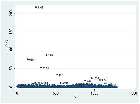
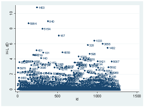
So far, we have seen the basic three diagnostic statistics: the Pearson residual, the deviance residual and the leverage (the hat value). They are the basic building blocks in logistic regression diagnostics. There are other diagnostic statistics that are used for different purposes. One important aspect of diagnostics is to identify observations with substantial impact on either the chi-square fit statistic or the deviance statistic. For example, we may want to know how much change in either the chi-square fit statistic or in the deviance statistic a single observation would cause. This leads to the dx2 and dd statistics. dx2 stands for the difference of chi-squares and dd stands for the difference of deviances. In Stata, we can simply use the predict command after the logit or logistic command to create these variables, as shown below. We can then visually inspect them. It is worth noticing that, first of all, these statistics are only so-called one-step approximation of the difference, not quite the exact difference, since it would be computationally too extensive to obtain exact difference for every observation. Secondly, Stata does all the diagnostic statistics for logistic regression using covariate patterns. Each observation will have exactly the same diagnostic statistics as all of the other observations in the same covariate pattern.
predict dx2, dx2
predict dd, dd
scatter dx2 id, mlab(snum)
scatter dd id, mlab(snum)
The observation with snum=1403 is obviously substantial in terms of both chi-square fit and the deviance fit statistic. For example, in the first plot, we see that dx2 is about 216 for this observation and below 100 for the rest of the observations. This means that when this observation is excluded from our analysis, the Pearson chi-square fit statistic will decrease by roughly 216. In the second plot, the observation with snum = 1403 will increase the deviance about 11. We can run two analysis and compare their Pearson chi-squares to see if this is the case.
logit hiqual avg_ed yr_rnd meals fullc yxfc

(Iterations omitted.)
Logit estimates Number of obs = 1158 LR chi2(5) = 933.71 Prob > chi2 = 0.0000 Log likelihood = -263.83452 Pseudo R2 = 0.6389 ------------------------------------------------------------------------------ hiqual | Coef. Std. Err. z P>|z| [95% Conf. Interval] -------------+---------------------------------------------------------------- avg_ed | 1.968948 .2850136 6.91 0.000 1.410332 2.527564 yr_rnd | -.5484941 .3680305 -1.49 0.136 -1.269821 .1728325 meals | -.0789775 .0079544 -9.93 0.000 -.0945677 -.0633872 fullc | .0499983 .01452 3.44 0.001 .0215397 .0784569 yxfc | -.1329371 .0325101 -4.09 0.000 -.1966557 -.0692185 _cons | -3.655163 1.016972 -3.59 0.000 -5.648392 -1.661935 ------------------------------------------------------------------------------ lfit Logistic model for hiqual, goodness-of-fit test number of observations = 1158 number of covariate patterns = 1152 Pearson chi2(1146) = 965.79 Prob > chi2 = 1.0000 logit hiqual avg_ed yr_rnd meals fullc yxfc if snum!=1403, nologLogit estimates Number of obs = 1157 LR chi2(5) = 943.15 Prob > chi2 = 0.0000 Log likelihood = -257.99083 Pseudo R2 = 0.6464 ------------------------------------------------------------------------------ hiqual | Coef. Std. Err. z P>|z| [95% Conf. Interval] -------------+---------------------------------------------------------------- avg_ed | 2.030088 .2915102 6.96 0.000 1.458739 2.601437 yr_rnd | -.7044717 .3864407 -1.82 0.068 -1.461882 .0529381 meals | -.0797143 .0080847 -9.86 0.000 -.0955601 -.0638686 fullc | .0504368 .0146263 3.45 0.001 .0217697 .0791038 yxfc | -.1078501 .0372207 -2.90 0.004 -.1808013 -.034899 _cons | -3.819562 1.035962 -3.69 0.000 -5.850011 -1.789114 ------------------------------------------------------------------------------ lfit Logistic model for hiqual, goodness-of-fit test number of observations = 1157 number of covariate patterns = 1151 Pearson chi2(1145) = 794.17 Prob > chi2 = 1.0000 di 965.79-794.17 171.62
It is not very close to 216, but they are in the same magnitude. This is because of the one-step approximation process that Stata uses. We can also look at the difference between deviances in a same way.
logit hiqual avg_ed yr_rnd meals fullc yxfc, nologLogit estimates Number of obs = 1158 LR chi2(5) = 933.71 Prob > chi2 = 0.0000 Log likelihood = -263.83452 Pseudo R2 = 0.6389 ------------------------------------------------------------------------------ hiqual | Coef. Std. Err. z P>|z| [95% Conf. Interval] -------------+---------------------------------------------------------------- avg_ed | 1.968948 .2850136 6.91 0.000 1.410332 2.527564 yr_rnd | -.5484941 .3680305 -1.49 0.136 -1.269821 .1728325 meals | -.0789775 .0079544 -9.93 0.000 -.0945677 -.0633872 fullc | .0499983 .01452 3.44 0.001 .0215397 .0784569 yxfc | -.1329371 .0325101 -4.09 0.000 -.1966557 -.0692185 _cons | -3.655163 1.016972 -3.59 0.000 -5.648392 -1.661935 ------------------------------------------------------------------------------ logit hiqual avg_ed yr_rnd meals fullc yxfc if snum!=1403, nologLogit estimates Number of obs = 1157 LR chi2(5) = 943.15 Prob > chi2 = 0.0000 Log likelihood = -257.99083 Pseudo R2 = 0.6464 ------------------------------------------------------------------------------ hiqual | Coef. Std. Err. z P>|z| [95% Conf. Interval] -------------+---------------------------------------------------------------- avg_ed | 2.030088 .2915102 6.96 0.000 1.458739 2.601437 yr_rnd | -.7044717 .3864407 -1.82 0.068 -1.461882 .0529381 meals | -.0797143 .0080847 -9.86 0.000 -.0955601 -.0638686 fullc | .0504368 .0146263 3.45 0.001 .0217697 .0791038 yxfc | -.1078501 .0372207 -2.90 0.004 -.1808013 -.034899 _cons | -3.819562 1.035962 -3.69 0.000 -5.850011 -1.789114 ------------------------------------------------------------------------------ di (263.83452 -257.99083)*2 11.68738
Since the deviance is simply 2 times the log likelihood, we can compute the difference of deviances as 2 times the difference in log likelihoods. When could it happen that an observation has great impact on fit statistics, but not too much impact on parameter estimates? This is actually the case for the observation with snum=1403, because its leverage is not very large. Notice that the the observation with snum=1403 has a fairly large residual. This means that the values for the independent variables of the observation are not in an extreme region, but the observed outcome for this point is very different from the predicted value. From the list of the observation below, we see that the percent of students receiving free or reduced-priced meals is about 100 percent, the avg_ed score is 2.19, and it is a year-around school. All things considered, we wouldn’t expect that this school is a high performance school. But its api score is 808, which is very high.
clist if snum==1403

Observation 243

        snum         1403        dnum          315     schqual         high      hiqual         high
      yr_rnd        yrrnd       meals          100      enroll          497        cred          low
     cred_ml          low     cred_hl          low       pared       medium    pared_ml       medium
    pared_hl            .       api00          808       api99          824        full           59
    some_col           28      awards           No         ell           27      avg_ed         2.19
       fullc    -29.12417        yxfc    -29.12417           p     .0046147      stdres     14.71427
          id          243          dv      3.27979         hat     .0037408         dx2     216.5097
          dd     10.79742
With information on school number and district number, we can find out to which school this observation corresponds. It turns out that this school is Kelso Elementary School in Inglewood that has been doing remarkably well. One can easily find many interesting articles about the school. Therefore, regression diagnostics help us to recognize those schools that are of interest to study by themselves.
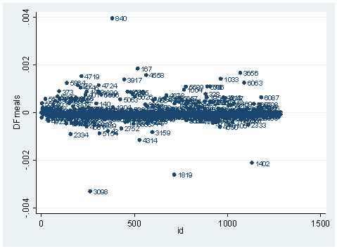
The last type of diagnostic statistics is related to coefficient sensitivity. It concerns how much impact each observation has on each parameter estimate. Similar to OLS regression, we also have dfbeta’s for logistic regression. A program called ldfbeta is available for download by using “search ldfbeta“. Like other diagnostic statistics for logistic regression, ldfbeta also uses one-step approximation. Unlike other logistic regression diagnostics in Stata, ldfbeta is at the individual observation level, instead of at the covariate pattern level. After either the logit or logistic command, we can simply issue the ldfbeta command. It can be used without any arguments, and in that case, dfbeta is calculated for each of the predictor variables. It will take some time since it is somewhat computationally intensive. Or we can specify a variable, as shown below. For example, suppose that we want to know how each individual observation affects the parameter estimate for the variable meals.
ldfbeta meals
DFmeals:   DFbeta(meals)

scatter DFmeals id, mlab(snum)
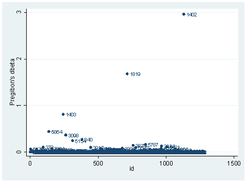
There is another statistic called Pregibon’s dbeta which is provides summary information of influence on parameter estimates of each individual observation (more precisely each covariate pattern). dbeta is very similar to Cook’s D in ordinary linear regression. This is more commonly used since it is much less computationally intensive. We can obtain dbeta using the predict command after the logit or logistic command.
predict dbeta, dbeta
scatter dbeta id, mlab(snum)
We have seen quite a few logistic regression diagnostic statistics. Now how large does each one have to be, to be considered influential? First of all, we always have to make our judgment based on our theory and our analysis. Secondly, there are some rule-of-thumb cutoffs when the sample size is large. These are shown below. When the sample size is large, the asymptotic distribution of some of the measures would follow some standard distribution. That is why we have these cutoff values, and why they only apply when the sample size is large enough. Usually, we would look at the relative magnitude of a statistic an observation has compared to others. That is, we look for data points that are farther away from most of the data points.
| Measure | Value |
| leverage (hat value) | >2 or 3 times of the average of leverage |
| abs(Pearson Residuals) | > 2 |
| abs(Deviance Residuals) | > 2 |
3.5 Common Numerical Problems with Logistic Regression
In this section, we are going to discuss some common numeric problems with logistic regression analysis.
When we have categorical predictor variables, we may run into a “zero-cells” problem. Let’s look at an example. In the data set hsb2, we have a variable called write for writing scores. For the purpose of illustration, we dichotomize this variable into two groups as a new variable called hw. Notice that one group is really small. With respect to another variable, ses, the crosstabulation shows that some cells have very few observations, and, in particular, the cell with hw = 1 and ses = low, the number of observations is zero. This will cause a computation issue when we run the logistic regression using hw as the dependent variable and ses as the predictor variable, as shown below.
use https://stats.idre.ucla.edu/stat/stata/notes/hsb2, clear
gen hw=write>=67
tab hw ses
| ses hw | low middle high | Total -----------+---------------------------------+---------- 0 | 47 93 53 | 193 1 | 0 2 5 | 7 -----------+---------------------------------+---------- Total | 47 95 58 | 200xi: logit hw i.ses, nolog i.ses _Ises_1-3 (naturally coded; _Ises_1 omitted)Logistic regression Number of obs = 200 LR chi2(2) = 7.22 Prob > chi2 = 0.0271 Log likelihood = -26.733291 Pseudo R2 = 0.1190------------------------------------------------------------------------------ hw | Coef. Std. Err. z P>|z| [95% Conf. Interval] -------------+---------------------------------------------------------------- _Ises_2 | 14.53384 . . . . . _Ises_3 | 16.01244 .8541783 18.75 0.000 14.33828 17.6866 _cons | -18.3733 .7146696 -25.71 0.000 -19.77402 -16.97257 ------------------------------------------------------------------------------ Note: 47 failures and 0 successes completely determined.
Notice that it takes more iterations to run this simple model and at the end, there is no standard error for the dummy variable _Ises_2. Stata also issues a warning at the end. So what has happened? The 47 failures in the warning note correspond to the observations in the cell with hw = 0 and ses = 1 as shown in the crosstabulation above. It is certain that the outcome will be 0 if the variable ses takes the value of 1 since there are no observations in the cell with hw=1 and ses =1. Although ses seems to be a good predictor, the empty cell causes the estimation procedure to fail. In fact, the odds ratio of each of the predictor variables is going to the roof:
logit, or
Logistic regression                               Number of obs   =        200
                                                  LR chi2(2)      =       7.22
                                                  Prob > chi2     =     0.0271
Log likelihood = -26.733291                       Pseudo R2       =     0.1190
------------------------------------------------------------------------------
hw | Odds Ratio Std. Err. z P>|z| [95% Conf. Interval]
-------------+----------------------------------------------------------------
_Ises_2 | 2051010 . . . . .
_Ises_3 | 8997355 7685345 18.75 0.000 1686696 4.80e+07
------------------------------------------------------------------------------
Note: 47 failures and 0 successes completely determined.
What do we do if a similar situation happens to our real-world data analysis? Two obvious options are available. One is to take this variable out of the regression model. It might not be a good option, but it could help in verifying the problem. The other option is to collapse across some of the categories to increase the cell size. For example, we can collapse the two lower categories of the variable ses into one category.
Here is a trivial example of perfect separation. Recall that our variable hw is created based on the writing score. So what happens when we use the variable write to predict hw? Of course, we will have a perfect prediction with hw= 1 if and only if write >=67. Therefore, if we try to run this logit model in Stata, we will not see any estimates but simply a message:
logit hw writeoutcome = write > 65 predicts data perfectly r(2000);
This is a very contrived example for the purpose of illustration.
3.6 Summary of Useful Commands
-
- linktest–performs a link test for model specification, in our case to check if logit is the right link function to use. This command is issued after the logit or logistic command.
- lfit–performs goodness-of-fit test, calculates either Pearson chi-square goodness-of-fit statistic or Hosmer-Lemeshow chi-square goodness-of-fit depending on if the group option is used.
- fitstat — is a post-estimation command that computes a variety of measures of fit.
- lsens — graphs sensitivity and specificity versus probability cutoff.
- lstat — displays summary statistics, including the classification table, sensitivity, and specificity.
- lroc — graphs and calculates the area under the ROC curve based on the model.
- listcoef–lists the estimated coefficients for a variety of regression models, including logistic regression.
- predict dbeta — Pregibon delta beta influence statistic
- predict deviance — deviance residual
- predict dx2 — Hosmer and Lemeshow change in chi-square influence statistic
- predict dd — Hosmer and Lemeshow change in deviance statistic
- predict hat — Pregibon leverage
- predict residual — Pearson residuals; adjusted for the covariate pattern
- predict rstandard — standardized Pearson residuals; adjusted for the covariate pattern
- ldfbeta — influence of each individual observation on the coefficient estimate ( not adjusted for the covariate pattern)
- graph with [weight=some_variable] option
- scatlog–produces scatter plot for logistic regression.
- boxtid–performs power transformation of independent variables and performs nonlinearity test.
References
Berry, W. D., and Feldman, S. (1985) Multiple Regression in Practice. Sage University Paper Series on Quantitative Applications in the Social Sciences, 07-050. Beverly Hill, CA: Sage.
Fox, John (1991) Regression Diagnostics. Sage University Paper Series on Quantitative Applications in the Social Sciences, 07-079. Newbury Park, CA: Sage.
Hosmer, D. and Lemeshw, S. (2000) Applied Logistic Regression, 2nd Edition, John Wiley & Sons, Inc.
Long and Freese, Regression Models for Categorical Dependent Variables Using Stata, 2nd Edition.
Menard, S. (1995) Applied Logistic Regression Analysis. Sage University Paper Series on Quantitative Applications in the Social Sciences, 07-106. Thousand Oaks, CA: Sage.
Pregibon, D. (1981) Logistic Regression Diagnostics, Annals of Statistics, Vol. 9, 705-724.

