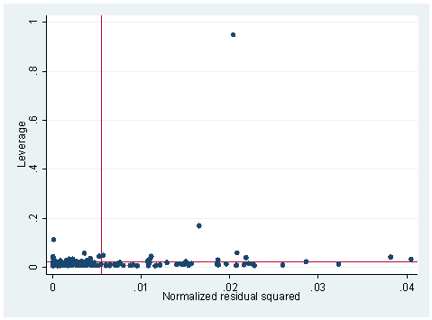
1. The following data set consists of measured weight, measured height, reported weight and reported height of some 200 people. You can get it from within Stata by typing use https://stats.idre.ucla.edu/stat/stata/webbooks/reg/davis We tried to build a model to predict measured weight by reported weight, reported height and measured height. We did an lvr2plot after the regression and here is what we have. Explain what you see in the graph and try to use other STATA commands to identify the problematic observation(s). What do you think the problem is and what is your solution?
use https://stats.idre.ucla.edu/stat/stata/webbooks/reg/davis
regress  measwt measht reptwt reptht
Source | SS df MS Number of obs = 181 ---------+------------------------------ F( 3, 177) = 1640.88 Model | 40891.9594 3 13630.6531 Prob > F = 0.0000 Residual | 1470.3279 177 8.30693727 R-squared = 0.9653 ---------+------------------------------ Adj R-squared = 0.9647 Total | 42362.2873 180 235.346041 Root MSE = 2.8822 ------------------------------------------------------------------------------ measwt | Coef. Std. Err. t P>|t| [95% Conf. Interval] ---------+-------------------------------------------------------------------- measht | -.9607757 .0260189 -36.926 0.000 -1.012123 -.9094285 reptwt | 1.01917 .0240778 42.328 0.000 .971654 1.066687 reptht | .8184156 .0419658 19.502 0.000 .7355979 .9012334 _cons | 24.8138 4.888302 5.076 0.000 15.16695 34.46065 ------------------------------------------------------------------------------lvr2plot
2. Using the data from the last exercise, what measure would you use if you want to know how much change an observation would make on a coefficient for a predictor? For example, show how much change would it be for the coefficient of predictor reptht if we omit observation 12 from our regression analysis? What are the other measures that you would use to assess the influence of an observation on regression? What are the cut-off values for them?
3. The following data file is called bbwt.dta and it is from Weisberg’s Applied Regression Analysis. You can obtain it from within Stata by typing use https://stats.idre.ucla.edu/stat/stata/webbooks/reg/bbwt It consists of the body weights and brain weights of some 60 animals. We want to predict the brain weight by body weight, that is, a simple linear regression of brain weight against body weight. Show what you have to do to verify the linearity assumption. If you think that it violates the linearity assumption, show some possible remedies that you would consider.
use https://stats.idre.ucla.edu/stat/stata/webbooks/reg/bbwt, clear
regress brainwt bodywt
Source | SS df MS Number of obs = 62 ---------+------------------------------ F( 1, 60) = 411.12 Model | 46067326.8 1 46067326.8 Prob > F = 0.0000 Residual | 6723217.18 60 112053.62 R-squared = 0.8726 ---------+------------------------------ Adj R-squared = 0.8705 Total | 52790543.9 61 865418.753 Root MSE = 334.74 ------------------------------------------------------------------------------ brainwt | Coef. Std. Err. t P>|t| [95% Conf. Interval] ---------+-------------------------------------------------------------------- bodywt | .9664599 .0476651 20.276 0.000 .8711155 1.061804 _cons | 91.00865 43.55574 2.089 0.041 3.884201 178.1331 ------------------------------------------------------------------------------
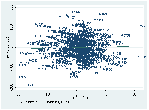
4. We did a regression analysis using the data file elemapi2 in chapter 2. Continuing with the analysis we did, we did an avplot here. Explain what an avplot is and what type of information you would get from the plot. If variable full were put in the model, would it be a significant predictor?
use https://stats.idre.ucla.edu/stat/stata/webbooks/reg/elemapi2, clear
regress api00 meals ell emer
Source | SS df MS Number of obs = 400 ---------+------------------------------ F( 3, 396) = 673.00 Model | 6749782.75 3 2249927.58 Prob > F = 0.0000 Residual | 1323889.25 396 3343.15467 R-squared = 0.8360 ---------+------------------------------ Adj R-squared = 0.8348 Total | 8073672.00 399 20234.7669 Root MSE = 57.82 ------------------------------------------------------------------------------ api00 | Coef. Std. Err. t P>|t| [95% Conf. Interval] ---------+-------------------------------------------------------------------- meals | -3.159189 .1497371 -21.098 0.000 -3.453568 -2.864809 ell | -.9098732 .1846442 -4.928 0.000 -1.272878 -.5468678 emer | -1.573496 .293112 -5.368 0.000 -2.149746 -.9972456 _cons | 886.7033 6.25976 141.651 0.000 874.3967 899.0098 ------------------------------------------------------------------------------avplot full, mlabel(snum)
5. The data set wage.dta is from a national sample of 6000 households with a male head earning less than $15,000 annually in 1966. You can get this data file by typing use https://stats.idre.ucla.edu/stat/stata/webbooks/reg/wage from within Stata. The data were classified into 39 demographic groups for analysis. We tried to predict the average hours worked by average age of respondent and average yearly non-earned income.
use https://stats.idre.ucla.edu/stat/stata/webbooks/reg/wage, clear
regress HRS AGE NEIN
Source | SS df MS Number of obs = 39 ---------+------------------------------ F( 2, 36) = 39.72 Model | 107205.109 2 53602.5543 Prob > F = 0.0000 Residual | 48578.1222 36 1349.39228 R-squared = 0.6882 ---------+------------------------------ Adj R-squared = 0.6708 Total | 155783.231 38 4099.5587 Root MSE = 36.734 ------------------------------------------------------------------------------ HRS | Coef. Std. Err. t P>|t| [95% Conf. Interval] ---------+-------------------------------------------------------------------- AGE | -8.281632 1.603736 -5.164 0.000 -11.53416 -5.029104 NEIN | .4289202 .0484882 8.846 0.000 .3305816 .5272588 _cons | 2321.03 57.55038 40.330 0.000 2204.312 2437.748 ------------------------------------------------------------------------------
Both predictors are significant. Now if we add ASSET to our predictors list, neither NEIN nor ASSET is significant.
regress HRS AGE NEIN ASSETSource | SS df MS Number of obs = 39 ---------+------------------------------ F( 3, 35) = 25.83 Model | 107317.64 3 35772.5467 Prob > F = 0.0000 Residual | 48465.5908 35 1384.73117 R-squared = 0.6889 ---------+------------------------------ Adj R-squared = 0.6622 Total | 155783.231 38 4099.5587 Root MSE = 37.212 ------------------------------------------------------------------------------ HRS | Coef. Std. Err. t P>|t| [95% Conf. Interval] ---------+-------------------------------------------------------------------- AGE | -8.007181 1.88844 -4.240 0.000 -11.84092 -4.173443 NEIN | .3338277 .337171 0.990 0.329 -.3506658 1.018321 ASSET | .0044232 .015516 0.285 0.777 -.027076 .0359223 _cons | 2314.054 63.22636 36.600 0.000 2185.698 2442.411 ------------------------------------------------------------------------------
Can you explain why?
6. Continue to use the previous data set. This time we want to predict the average hourly wage by average percent of white respondents. Carry out the regression analysis and list the STATA commands that you can use to check for heteroscedasticity. Explain the result of your test(s).
Now we want build another model to predict the average percent of white respondents by the average hours worked. Repeat the analysis you performed on the previous regression model. Explain your results.
7. We have a data set that consists of volume, diameter and height of some objects. Someone did a regression of volume on diameter and height.
use https://stats.idre.ucla.edu/stat/stata/webbooks/reg/tree, clear
regress vol dia height
Source | SS df MS Number of obs = 31 ---------+------------------------------ F( 2, 28) = 254.97 Model | 7684.16254 2 3842.08127 Prob > F = 0.0000 Residual | 421.921306 28 15.0686181 R-squared = 0.9480 ---------+------------------------------ Adj R-squared = 0.9442 Total | 8106.08385 30 270.202795 Root MSE = 3.8818 ------------------------------------------------------------------------------ vol | Coef. Std. Err. t P>|t| [95% Conf. Interval] ---------+-------------------------------------------------------------------- dia | 4.708161 .2642646 17.816 0.000 4.166839 5.249482 height | .3392513 .1301512 2.607 0.014 .0726487 .6058538 _cons | -57.98766 8.638225 -6.713 0.000 -75.68226 -40.29306 ------------------------------------------------------------------------------
Explain what tests you can use to detect model specification errors and if there is any, your solution to correct it.

