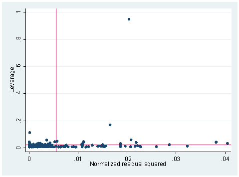
1. The following data set consists of measured weight, measured height, reported weight and reported height of some 200 people. We tried to build a model to predict measured weight by reported weight, reported height and measured height. We did an lvr2plot after the regression and here is what we have. Explain what you see in the graph and try to use other STATA commands to identify the problematic observation(s). What do you think the problem is and what is your solution?
use davis, clear
regress  measwt measht reptwt reptht

Source |       SS       df       MS                    Number of obs =     181
---------+------------------------------               F(  3,   177) = 1640.88
   Model |  40891.9594     3  13630.6531               Prob > F      =  0.0000
Residual |   1470.3279   177  8.30693727               R-squared     =  0.9653
---------+------------------------------               Adj R-squared =  0.9647
   Total |  42362.2873   180  235.346041               Root MSE      =  2.8822

------------------------------------------------------------------------------
  measwt |      Coef.   Std. Err.       t     P>|t|       [95% Conf. Interval]
---------+--------------------------------------------------------------------
  measht |  -.9607757   .0260189    -36.926   0.000      -1.012123   -.9094285
  reptwt |    1.01917   .0240778     42.328   0.000        .971654    1.066687
  reptht |   .8184156   .0419658     19.502   0.000       .7355979    .9012334
   _cons |    24.8138   4.888302      5.076   0.000       15.16695    34.46065
------------------------------------------------------------------------------

lvr2plot
Answer:
lvr2plot is the leverage against residual squared plot. The upper left corner of the plot will be points that are high in leverage and the lower right corner will be points that are high in the absolute of residuals. The upper right portion will be those points that are both high in leverage and in the absolute of residuals. There is one point in this plot that stands out so much differently from any other point. There are many ways of figuring out what this point is. First of all, graphically, we can add an option in our lvr2plot command to see which observation is associated with the extreme point on the plot.
lvr2plot, ml(subject)
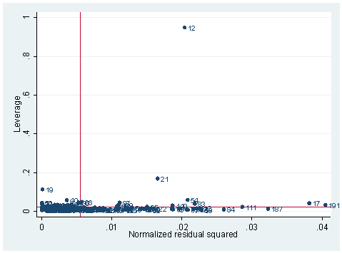
There are also numerical measures that we can deploy. Since it is obviously very high on leverage, we can first generate leverage and list the extreme ones.
predict l, leverage
hilo l  measwt measht reptwt reptht  subject, high show(5)
5 highest observations on l

        l     measwt     measht     reptwt     reptht    subject
0578113         65        187         67        188         40
0596073        102        185        107        185         54
1136993         76        197         75        200         19
1702566        119        180        124        178         21
9481246        166         57         56        163         12
The other way is to use Cook’s D since Cook’s D is the combination of leverage and residual.
predict c, cooksd
hilo c  measwt measht reptwt reptht  subject, high show(5)
5 highest observations on c

        c     measwt     measht     reptwt     reptht    subject
0619987        102        185        107        185         54
0628549         88        185         93        188        191
0779325         92        187        101        185         17
1808358        119        180        124        178         21
 317.8551        166         57         56        163         12
We can also look at studentized residuals.
predict rstu, rstu
hilo  rstu measwt measht reptwt reptht subject, show(5)
5 lowest and highest observations on rstu

     rstu     measwt     measht     reptwt     reptht    subject
-2.772892         88        185         93        188        191
-2.703085         92        187        101        185         17
-2.305224         84        183         90        183        111
-2.023018         53        169         52        175         83
-1.994573        102        185        107        185         54

     rstu     measwt     measht     reptwt     reptht    subject
 2.030575         58        161         51        159          2
 2.031815         75        172         70        169         59
 2.176899         60        167         55        163         84
 2.440577         60        172         55        168        187
 10.67515        166         57         56        163         12
In all of the above, we see that subject 12 is a problematic point. Is it an entry error? Yes. Apparently for subject 12 the measured weight has been switched with measured height. We can be very much sure on this case. Therefore, we can switch them back. We then perform the same analysis again.
replace measwt=57 if  subject==12
(1 real change made)

replace measht=166 if subject==12
(1 real change made)

list  subject measwt  measht reptwt reptht in 12/12

       subject     measwt     measht     reptwt     reptht
 12.        59         75        172         70        169

regress  measwt measht reptwt reptht

  Source |       SS       df       MS                  Number of obs =     181
---------+------------------------------               F(  3,   177) = 2085.02
   Model |  31551.0849     3  10517.0283               Prob > F      =  0.0000
Residual |  892.804651   177  5.04409407               R-squared     =  0.9725
---------+------------------------------               Adj R-squared =  0.9720
   Total |  32443.8895   180  180.243831               Root MSE      =  2.2459

------------------------------------------------------------------------------
  measwt |      Coef.   Std. Err.       t     P>|t|       [95% Conf. Interval]
---------+--------------------------------------------------------------------
  measht |  -.0364477    .088613     -0.411   0.681      -.2113216    .1384262
  reptwt |    .963793   .0194467     49.561   0.000       .9254157     1.00217
  reptht |   .0225427   .0811435      0.278   0.781      -.1375904    .1826759
   _cons |   4.821849   4.242671      1.137   0.257      -3.550881    13.19458
------------------------------------------------------------------------------
We now see that both measured height and reported height are no longer significant predictors. This is because that the predictors are collinear to each other since we have corrected the entry error. Let’s do another regression with only reported weight as a single predictor. Notice that adjusted R-square is actually the highest among all the regression analysis we have done so far. This shows that data entry error could really distort the regression analysis sometimes.
regress  measwt reptwt

  Source |       SS       df       MS                  Number of obs =     181
---------+------------------------------               F(  1,   179) = 6315.72
   Model |  31549.7087     1  31549.7087               Prob > F      =  0.0000
Residual |  894.180797   179  4.99542345               R-squared     =  0.9724
---------+------------------------------               Adj R-squared =  0.9723
   Total |  32443.8895   180  180.243831               Root MSE      =   2.235

------------------------------------------------------------------------------
  measwt |      Coef.   Std. Err.       t     P>|t|       [95% Conf. Interval]
---------+--------------------------------------------------------------------
  reptwt |   .9569886   .0120419     79.472   0.000       .9332262    .9807509
   _cons |   2.847071   .8081664      3.523   0.001       1.252311     4.44183
------------------------------------------------------------------------------
2. Continue with the first model we run in our last exercise. What measure and its corresponding STATA command would you use if you want to know how much change an observation would make on a predictor? For example, how much change would it be for the coefficient of predictor reptht if we omit observation 12 from our regression analysis? What are the other measures that you would use to assess the strength of an observation on regression? What are the commonly suggested cut-off values for them?
Answer: The measure that measures how much impact each observation has on a particular predictor is DFBETAs. The DFBETA for a predictor and for a particular observation is the difference between the regression coefficient calculated for all of the data and the regression coefficient calculated with the observation deleted, scaled by the standard error calculated with the observation deleted. The cut-off value for DFBETAs is 2/sqrt(n), where n is the number of observations. In our case, it will be the absolute value of DFBETAs greater than 2/sqrt(181)=.14866. From our list below, we can see we have several troublesome points with observation 12 the most troublesome one. For observation 12, the DFreptht is 24.25463. That means that including observation 12 in the regression, the regression coefficient for reptht will increase by about 24 times the standard error than the case with the observation excluded.
dfbeta
DFmeasht:  DFbeta(measht)
DFreptwt:  DFbeta(reptwt)
DFreptht:  DFbeta(reptht)

hilo  DFreptht measwt measht reptwt reptht subject, show(5)
5 lowest and highest observations on DFreptht

 DFreptht     measwt     measht     reptwt     reptht    subject
-.3410896         53        169         52        175         83
-.2115161         88        185         93        188        191
-.1834869         59        182         61        183         86
-.1629187         65        187         67        188         40
-.1510676         79        179         79        171        112

 DFreptht     measwt     measht     reptwt     reptht    subject
0904913         63        160         64        158         78
1255461         69        167         73        165        122
1791834         85        191         83        188        140
4119168        119        180        124        178         21
 24.25463        166         57         56        163         12
DFBETAs are calculation intensive as it is for computed each predictor and each observation. DFITS and Cook’s D, on the other hand, are summary information of the influence (leverage and residual) and are much less computation intensive. For example, we can look at DFITS after the regression, similar to what we did in Exercise 1. The cut-off values of DFITS and Cook’s D is 2*sqrt(k/n) and 4/n respectively. Observations with DFITS or Cook’s D value greater than these cut-off values deserve further investigation.
3. The following data file is called bbwt.dta and it is from Weisberg’s Applied Regression Analysis. It consists of the body weights and brain weight of some 60 animals. We want to predict the brain weight by body weight, that is, a simple linear regression of brain weight against body weight. Show what you have to do to verify the linearity assumption. If you think that it violates the linearity assumption, show some possible remedies that you would consider.
use bbwt, clearregress brainwt bodywtSource | SS df MS Number of obs = 62 ---------+------------------------------ F( 1, 60) = 411.12 Model | 46067326.8 1 46067326.8 Prob > F = 0.0000 Residual | 6723217.18 60 112053.62 R-squared = 0.8726 ---------+------------------------------ Adj R-squared = 0.8705 Total | 52790543.9 61 865418.753 Root MSE = 334.74 ------------------------------------------------------------------------------ brainwt | Coef. Std. Err. t P>|t| [95% Conf. Interval] ---------+-------------------------------------------------------------------- bodywt | .9664599 .0476651 20.276 0.000 .8711155 1.061804 _cons | 91.00865 43.55574 2.089 0.041 3.884201 178.1331 ------------------------------------------------------------------------------
Answer: In general, we can use acprplot to verify the linearity assumption against a predictor. For example, we can do after the regression above the acprplot against our only predictor bodywt.
acprplot bodywt, mspline
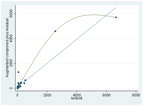
The graph does not look very linear. In our chapter, we did some logarithm transformations. We’ll try it here and the results are shown below. Notice the plot is much nicer this time. The adjusted R-square is also up by .05.
gen lbdwt=log(bodywt)

gen lbrwt=log(brainwt)

regress   lbrwt lbdwt

  Source |       SS       df       MS                  Number of obs =      62
---------+------------------------------               F(  1,    60) =  697.42
   Model |  336.188605     1  336.188605               Prob > F      =  0.0000
Residual |  28.9226087    60  .482043478               R-squared     =  0.9208
---------+------------------------------               Adj R-squared =  0.9195
   Total |  365.111213    61  5.98542973               Root MSE      =  .69429

------------------------------------------------------------------------------
   lbrwt |      Coef.   Std. Err.       t     P>|t|       [95% Conf. Interval]
---------+--------------------------------------------------------------------
   lbdwt |   .7516861   .0284635     26.409   0.000       .6947507    .8086216
   _cons |   2.134788   .0960432     22.227   0.000       1.942673    2.326903
------------------------------------------------------------------------------

acprplot  lbdwt, mspline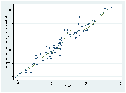
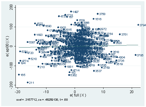
4. We did a regression analysis using data file elemapi in chapter 2. Continuing with the analysis we did, we did an avplot here. Explain what an avplot is and how you would interpret the avplot below. If full were put in the model, would it be a significant predictor?
use https://stats.idre.ucla.edu/stat/stata/webbooks/reg/elemapi2, clear
regress api00 meals ell emer
Source | SS df MS Number of obs = 400 ---------+------------------------------ F( 3, 396) = 673.00 Model | 6749782.75 3 2249927.58 Prob > F = 0.0000 Residual | 1323889.25 396 3343.15467 R-squared = 0.8360 ---------+------------------------------ Adj R-squared = 0.8348 Total | 8073672.00 399 20234.7669 Root MSE = 57.82 ------------------------------------------------------------------------------ api00 | Coef. Std. Err. t P>|t| [95% Conf. Interval] ---------+-------------------------------------------------------------------- meals | -3.159189 .1497371 -21.098 0.000 -3.453568 -2.864809 ell | -.9098732 .1846442 -4.928 0.000 -1.272878 -.5468678 emer | -1.573496 .293112 -5.368 0.000 -2.149746 -.9972456 _cons | 886.7033 6.25976 141.651 0.000 874.3967 899.0098 ------------------------------------------------------------------------------avplot full, mlabel(snum)
Answer: A group of points can be jointly influential. An avplot is an attractive graphic method to present multiple influential points on a predictor. What we are looking for in an avplot are those points that can exert substantial change to the regression line. For example, in the plot above, the observation with school number 211 is very low at the left corner of the plot. Deleting it would flatten the regression line a lot, in other words, it would decrease the regression coefficient for variable full significantly. You can compare the regression that includes the variable full and the entire data set and the model without the observation with snum 211.
regress api00 meals ell emer full

  Source |       SS       df       MS                  Number of obs =     400
---------+------------------------------               F(  4,   395) =  504.18
   Model |  6751342.63     4  1687835.66               Prob > F      =  0.0000
Residual |  1322329.37   395  3347.66928               R-squared     =  0.8362
---------+------------------------------               Adj R-squared =  0.8346
   Total |  8073672.00   399  20234.7669               Root MSE      =  57.859

------------------------------------------------------------------------------
   api00 |      Coef.   Std. Err.       t     P>|t|       [95% Conf. Interval]
---------+--------------------------------------------------------------------
   meals |  -3.156558   .1498877    -21.059   0.000      -3.451236   -2.861881
     ell |  -.8981675   .1855628     -4.840   0.000      -1.262982   -.5333532
    emer |  -1.225015     .58877     -2.081   0.038       -2.38253   -.0675008
    full |   .3157712   .4625914      0.683   0.495      -.5936778     1.22522
   _cons |   855.0671   46.76702     18.284   0.000       763.1237    947.0105
------------------------------------------------------------------------------

regress api00 meals ell emer  full if snum !=211

  Source |       SS       df       MS                  Number of obs =     399
---------+------------------------------               F(  4,   394) =  513.16
   Model |  6715948.02     4  1678987.01               Prob > F      =  0.0000
Residual |  1289106.10   394  3271.84289               R-squared     =  0.8390
---------+------------------------------               Adj R-squared =  0.8373
   Total |  8005054.12   398  20113.2013               Root MSE      =   57.20

------------------------------------------------------------------------------
   api00 |      Coef.   Std. Err.       t     P>|t|       [95% Conf. Interval]
---------+--------------------------------------------------------------------
   meals |  -3.164431   .1482011    -21.352   0.000      -3.455795   -2.873067
     ell |  -.8930366   .1834563     -4.868   0.000      -1.253712   -.5323609
    emer |  -1.411583    .585001     -2.413   0.016      -2.561697   -.2614692
    full |   .1213333   .4613751      0.263   0.793      -.7857315    1.028398
   _cons |   874.6425   46.64066     18.753   0.000       782.9468    966.3382
------------------------------------------------------------------------------
Of course, there are other points that are in similar nature as the observation with snum 211 shown in the avplot that are worth paying more attention to. On the other hand, if we look at the t-value on top of the avplot, it is only 68. The p-value corresponding to it will be the probability for t-distribution with degree of freedom being the total degree of freedom. :
di tprob(399, .683)
49500322
which is not significant. The equation on top of the avplot is actually the regression coefficient and its standard error if the variable were a predictor. In our regression which includes full and all the data, we see that coefficient for full is .3157712 and the standard error for it is .4625914. They are exactly the same as shown on top of the avplot.
5. The data set wage.dta is from a national sample of 6000 households with a male head earning less than $15,000 annually in 1966. The data were classified into 39 demographic groups for analysis. We tried to predict the average hours worked by average age of respondent and average yearly non-earned income.
use wage, clear
regress HRS AGE NEIN
Source | SS df MS Number of obs = 39 ---------+------------------------------ F( 2, 36) = 39.72 Model | 107205.109 2 53602.5543 Prob > F = 0.0000 Residual | 48578.1222 36 1349.39228 R-squared = 0.6882 ---------+------------------------------ Adj R-squared = 0.6708 Total | 155783.231 38 4099.5587 Root MSE = 36.734 ------------------------------------------------------------------------------ HRS | Coef. Std. Err. t P>|t| [95% Conf. Interval] ---------+-------------------------------------------------------------------- AGE | -8.281632 1.603736 -5.164 0.000 -11.53416 -5.029104 NEIN | .4289202 .0484882 8.846 0.000 .3305816 .5272588 _cons | 2321.03 57.55038 40.330 0.000 2204.312 2437.748 ------------------------------------------------------------------------------
Both predictors are significant. Now if we add ASSET to our predictors list, neither NEIN nor ASSET is significant.
regress HRS AGE NEIN ASSETSource | SS df MS Number of obs = 39 ---------+------------------------------ F( 3, 35) = 25.83 Model | 107317.64 3 35772.5467 Prob > F = 0.0000 Residual | 48465.5908 35 1384.73117 R-squared = 0.6889 ---------+------------------------------ Adj R-squared = 0.6622 Total | 155783.231 38 4099.5587 Root MSE = 37.212 ------------------------------------------------------------------------------ HRS | Coef. Std. Err. t P>|t| [95% Conf. Interval] ---------+-------------------------------------------------------------------- AGE | -8.007181 1.88844 -4.240 0.000 -11.84092 -4.173443 NEIN | .3338277 .337171 0.990 0.329 -.3506658 1.018321 ASSET | .0044232 .015516 0.285 0.777 -.027076 .0359223 _cons | 2314.054 63.22636 36.600 0.000 2185.698 2442.411 ------------------------------------------------------------------------------
Can you explain why?
Answer: If we look at our data set more carefully, for example, we can do a describe at the beginning of regression analysis, we would notice that variable NEIN and ASSET are very closed related. Therefore, we would expect that these two variables are strongly correlated. We can also do a scatter plot to check on this. Here is what we have done:
describe NEIN ASSETstorage display value variable name type format label variable label ------------------------------------------------------------------------------- NEIN float %9.0g Average yearly non-earned income ASSET float %9.0g Average family asset holdings (Bank account, etc.) ($)twoway (scatter NEIN ASSET) (lfit NEIN ASSET)
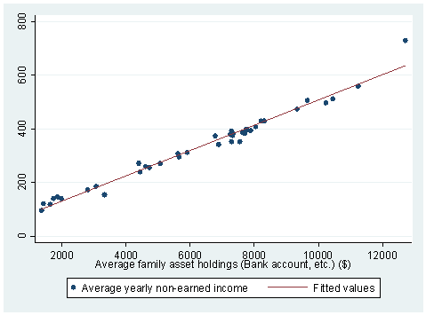
Another useful command introduced in this chapter is vif.
regress HRS AGE NEIN
(Output is shown above.)

vif

Variable |      VIF      1/VIF
---------+----------------------
     AGE |      1.29    0.774467
    NEIN |      1.29    0.774467
---------+----------------------
Mean VIF |      1.29

regress HRS AGE NEIN ASSET
(Output is shown above.)

vif

Variable |      VIF      1/VIF
---------+----------------------
    NEIN |     60.84    0.016436
   ASSET |     56.07    0.017836
     AGE |      1.74    0.573178
---------+----------------------
Mean VIF |     39.55
So we see that in the first regression, there is no evidence of collinearity since the variance inflation factors are fairly small. But in the second regression analysis, the vif for NEIN and ASSET jumped up to around 60, which indicates strongly the appearance of collinearity among the predictors. The collinearity can also be detected by using the command collin.
collin  NEIN ASSET AGE

  Collinearity Diagnostics

                        SQRT                           Cond
  Variable       VIF    VIF    Tolerance  Eigenval     Index
-------------------------------------------------------------
      NEIN     60.84    7.80    0.0164     2.2855     1.0000
     ASSET     56.07    7.49    0.0178     0.7059     1.7994
       AGE      1.74    1.32    0.5732     0.0086    16.3386
-------------------------------------------------------------
  Mean VIF     39.55              Condition Number   16.3386
6. Continue to use the previous data set. This time we want to predict the average hourly wage by the average percent of white respondents. Carry out the regression analysis and list the STATA commands that you can use to check for heteroscedasticity. Explain the results of the test(s).
use wage, clear
regress  RATE RACE

  Source |       SS       df       MS                  Number of obs =      31
---------+------------------------------               F(  1,    29) =   22.82
   Model |  2.16442894     1  2.16442894               Prob > F      =  0.0000
Residual |  2.75013286    29  .094832168               R-squared     =  0.4404
---------+------------------------------               Adj R-squared =  0.4211
   Total |  4.91456181    30  .163818727               Root MSE      =  .30795

------------------------------------------------------------------------------
    RATE |      Coef.   Std. Err.       t     P>|t|       [95% Conf. Interval]
---------+--------------------------------------------------------------------
    RACE |  -.0142697   .0029869     -4.777   0.000      -.0203786   -.0081608
   _cons |   3.367147   .1261571     26.690   0.000       3.109127    3.625168
------------------------------------------------------------------------------
hettest

Cook-Weisberg test for heteroscedasticity using fitted values of RATE
     Ho: Constant variance
         chi2(1)      =      0.42
         Prob > chi2  =      0.5186

whitetst
(8 missing values generated)
(8 missing values generated)

White's general test statistic :  .5617374  Chi-sq( 2)  P-value =  .7551
rvfplot
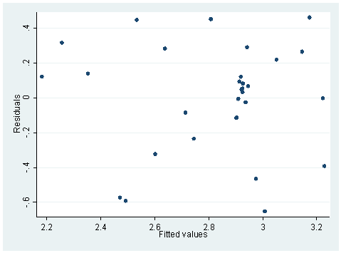
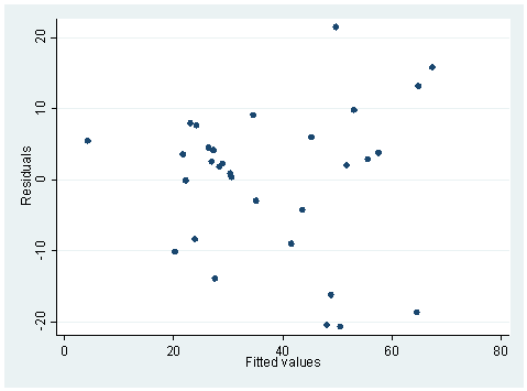
The hettest and whitetst are based on the null hypothesis that the variance is constant. Therefore, when the probability is large, we will accept the null hypothesis of constant variance. The rvfplot also shows that the variance across fitted values does not change a lot, as overall speaking we see a band of equal width. On the other hand, the regression below is different. Both hettest and whitetst are significant, indicating heteroscedasticity. This can also be seen from the rvfplot below, we see that the band is getting wider to the right.
regress RACE HRS

  Source |       SS       df       MS                  Number of obs =      31
---------+------------------------------               F(  1,    29) =   65.14
   Model |  7355.07438     1  7355.07438               Prob > F      =  0.0000
Residual |   3274.4589    29  112.912376               R-squared     =  0.6919
---------+------------------------------               Adj R-squared =  0.6813
   Total |  10629.5333    30  354.317776               Root MSE      =  10.626

------------------------------------------------------------------------------
    RACE |      Coef.   Std. Err.       t     P>|t|       [95% Conf. Interval]
---------+--------------------------------------------------------------------
     HRS |  -.2801356   .0347093     -8.071   0.000       -.351124   -.2091472
   _cons |   639.3401   74.53629      8.578   0.000       486.8963    791.7839
------------------------------------------------------------------------------

hettest

Cook-Weisberg test for heteroscedasticity using fitted values of RACE
     Ho: Constant variance
         chi2(1)      =      6.60
         Prob > chi2  =      0.0102

whitetst

White's general test statistic :  7.889606  Chi-sq( 2)  P-value =  .0194

rvfplot
7. We have a data set that consists of volume, diameter and height of some objects. Someone did a regression of volume on diameter and height.
use tree, clear
regress vol dia height
Source | SS df MS Number of obs = 31 ---------+------------------------------ F( 2, 28) = 254.97 Model | 7684.16254 2 3842.08127 Prob > F = 0.0000 Residual | 421.921306 28 15.0686181 R-squared = 0.9480 ---------+------------------------------ Adj R-squared = 0.9442 Total | 8106.08385 30 270.202795 Root MSE = 3.8818 ------------------------------------------------------------------------------ vol | Coef. Std. Err. t P>|t| [95% Conf. Interval] ---------+-------------------------------------------------------------------- dia | 4.708161 .2642646 17.816 0.000 4.166839 5.249482 height | .3392513 .1301512 2.607 0.014 .0726487 .6058538 _cons | -57.98766 8.638225 -6.713 0.000 -75.68226 -40.29306 ------------------------------------------------------------------------------
Explain what tests you can use to detect model specification errors and if there is any, your solution to correct it.
Answer: We can use linktest and ovtest to detect model specification errors.
linktest

  Source |       SS       df       MS                  Number of obs =      31
---------+------------------------------               F(  2,    28) =  594.19
   Model |  7919.48998     2  3959.74499               Prob > F      =  0.0000
Residual |  186.593864    28  6.66406657               R-squared     =  0.9770
---------+------------------------------               Adj R-squared =  0.9753
   Total |  8106.08385    30  270.202795               Root MSE      =  2.5815

------------------------------------------------------------------------------
     vol |      Coef.   Std. Err.       t     P>|t|       [95% Conf. Interval]
---------+--------------------------------------------------------------------
    _hat |   .3606632   .1115454      3.233   0.003       .1321728    .5891537
  _hatsq |   .0094227   .0015856      5.942   0.000       .0061746    .0126707
   _cons |   8.376438   1.729554      4.843   0.000       4.833608    11.91927
------------------------------------------------------------------------------

ovtest

Ramsey RESET test using powers of the fitted values of vol
       Ho:  model has no omitted variables
                  F(3, 25) =     11.54
                  Prob > F =      0.0001
For linktest we look for p-value for the square term and both the linktest and ovtest are significant indicating that our model is not specified correctly. It is actually easy to understand in this case, since we look for the relationship between volume, which is 3-dimensional and diameter and height, which are 1-dimensional. So it is reasonable to put in higher degree terms. One solution is to put the squared diameter term into our regression as shown below. Both the linktest and ovtest are no longer significant.
gen dia2=dia*dia

regress  vol dia dia2 height

  Source |       SS       df       MS                  Number of obs =      31
---------+------------------------------               F(  3,    27) =  383.20
   Model |  7920.07197     3  2640.02399               Prob > F      =  0.0000
Residual |  186.011883    27    6.889329               R-squared     =  0.9771
---------+------------------------------               Adj R-squared =  0.9745
   Total |  8106.08385    30  270.202795               Root MSE      =  2.6248

------------------------------------------------------------------------------
     vol |      Coef.   Std. Err.       t     P>|t|       [95% Conf. Interval]
---------+--------------------------------------------------------------------
     dia |  -2.885077   1.309851     -2.203   0.036      -5.572669   -.1974846
    dia2 |   .2686224   .0459048      5.852   0.000       .1744335    .3628112
  height |   .3763873    .088232      4.266   0.000       .1953502    .5574244
   _cons |  -9.920417   10.07912     -0.984   0.334      -30.60105    10.76022
------------------------------------------------------------------------------
linktest Source | SS df MS Number of obs = 31 ---------+------------------------------ F( 2, 28) = 596.13 Model | 7920.08338 2 3960.04169 Prob > F = 0.0000 Residual | 186.00047 28 6.64287391 R-squared = 0.9771 ---------+------------------------------ Adj R-squared = 0.9754 Total | 8106.08385 30 270.202795 Root MSE = 2.5774 ------------------------------------------------------------------------------ vol | Coef. Std. Err. t P>|t| [95% Conf. Interval] ---------+-------------------------------------------------------------------- _hat | 1.004811 .1199563 8.376 0.000 .7590915 1.25053 _hatsq | -.0000621 .0015027 -0.041 0.967 -.0031403 .0030161 _cons | -.0727509 2.019028 -0.036 0.972 -4.208542 4.06304 ------------------------------------------------------------------------------ ovtest Ramsey RESET test using powers of the fitted values of vol Ho: model has no omitted variables F(3, 24) = 0.43 Prob > F = 0.7312

