Chapter Outline
- 2.0 Regression Diagnostics
- 2.1 Unusual and Influential data
- 2.2 Checking Normality of Residuals
- 2.3 Checking Homoscedasticity
- 2.4 Checking for Multicollinearity
- 2.5 Checking Linearity
- 2.6 Model Specification
- 2.7 Issues of Independence
- 2.8 Summary
- 2.9 Self assessment
- 2.10 For more information
2.0 Regression Diagnostics
In the previous chapter, we learned how to do ordinary linear regression with Stata, concluding with methods for examining the distribution of our variables. Without verifying that your data have met the assumptions underlying OLS regression, your results may be misleading. This chapter will explore how you can use Stata to check on how well your data meet the assumptions of OLS regression. In particular, we will consider the following assumptions.
- Linearity – the relationships between the predictors and the outcome variable should be linear
- Normality – the errors should be normally distributed – technically normality is necessary only for hypothesis tests to be valid, estimation of the coefficients only requires that the errors be identically and independently distributed
- Homogeneity of variance (homoscedasticity) – the error variance should be constant
- Independence – the errors associated with one observation are not correlated with the errors of any other observation
- Errors in variables – predictor variables are measured without error (we will cover this in Chapter 4)
- Model specification – the model should be properly specified (including all relevant variables, and excluding irrelevant variables)
Additionally, there are issues that can arise during the analysis that, while strictly speaking are not assumptions of regression, are none the less, of great concern to data analysts.
- Influence – individual observations that exert undue influence on the coefficients
- Collinearity – predictors that are highly collinear, i.e., linearly related, can cause problems in estimating the regression coefficients.
Many graphical methods and numerical tests have been developed over the years for regression diagnostics. Stata has many of these methods built-in, and others are available that can be downloaded over the internet. In particular, Nicholas J. Cox (University of Durham) has produced a collection of convenience commands which can be downloaded from SSC (ssc install commandname). These commands include indexplot, rvfplot2, rdplot, qfrplot and ovfplot. In this chapter, we will explore these methods and show how to verify regression assumptions and detect potential problems using Stata.
2.1 Unusual and influential data
A single observation that is substantially different from all other observations can make a large difference in the results of your regression analysis. If a single observation (or small group of observations) substantially changes your results, you would want to know about this and investigate further. There are three ways that an observation can be unusual.
Outliers: In linear regression, an outlier is an observation with large residual. In other words, it is an observation whose dependent-variable value is unusual given its values on the predictor variables. An outlier may indicate a sample peculiarity or may indicate a data entry error or other problem.
Leverage: An observation with an extreme value on a predictor variable is called a point with high leverage. Leverage is a measure of how far an observation deviates from the mean
of that variable. These leverage points can have an effect on the estimate of regression coefficients.
Influence: An observation is said to be influential if removing the observation substantially changes the estimate of coefficients. Influence can be thought of as the product of leverage and outlierness.
How can we identify these three types of observations? Let’s look at an example dataset called crime. This dataset appears in Statistical Methods for Social Sciences, Third Edition by Alan Agresti and Barbara Finlay (Prentice Hall, 1997). The variables are state id (sid), state name (state), violent crimes per 100,000 people (crime), murders per 1,000,000 (murder), the percent of the population living in metropolitan areas (pctmetro), the percent of the population that is white (pctwhite), percent of population with a high school education or above (pcths), percent of population living under poverty line (poverty), and percent of population that are single parents (single).
use https://stats.idre.ucla.edu/stat/stata/webbooks/reg/crime
	(crime data from agresti & finlay - 1997)

describe

Contains data from crime.dta
  obs:            51                          crime data from agresti &
                                                finlay - 1997
 vars:            11                          6 Feb 2001 13:52
 size:         2,295 (98.9% of memory free)
-------------------------------------------------------------------------------
   1. sid       float  %9.0g
   2. state     str3   %9s
   3. crime     int    %8.0g                  violent crime rate
   4. murder    float  %9.0g                  murder rate
   5. pctmetro  float  %9.0g                  pct metropolitan
   6. pctwhite  float  %9.0g                  pct white
   7. pcths     float  %9.0g                  pct hs graduates
   8. poverty   float  %9.0g                  pct poverty
   9. single    float  %9.0g                  pct single parent
-------------------------------------------------------------------------------
Sorted by:

summarize crime murder pctmetro pctwhite pcths poverty single

Variable |     Obs        Mean   Std. Dev.       Min        Max
---------+-----------------------------------------------------
   crime |      51    612.8431   441.1003         82       2922
  murder |      51    8.727451   10.71758        1.6       78.5
pctmetro |      51     67.3902   21.95713         24        100
pctwhite |      51    84.11569   13.25839       31.8       98.5
   pcths |      51    76.22353   5.592087       64.3       86.6
 poverty |      51    14.25882   4.584242          8       26.4
  single |      51    11.32549   2.121494        8.4       22.1
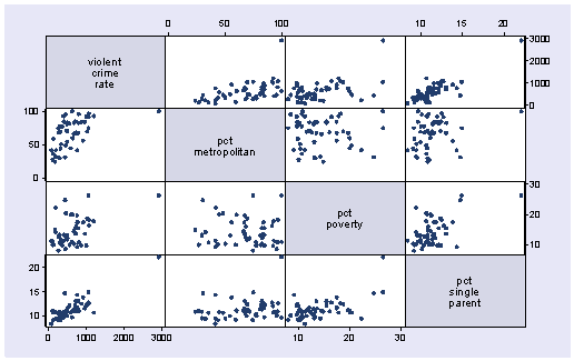
Let’s say that we want to predict crime by pctmetro, poverty, and single. That is to say, we want to build a linear regression model between the response variable crime and the independent variables pctmetro, poverty and single. We will first look at the scatter plots of crime against each of the predictor variables before the regression analysis so we will have some ideas about potential problems. We can create a scatterplot matrix of these variables as shown below.
graph matrix crime pctmetro poverty single
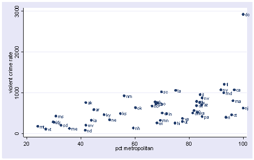
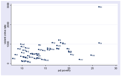
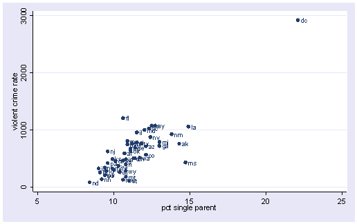
The graphs of crime with other variables show some potential problems. In every plot, we see a data point that is far away from the rest of the data points. Let’s make individual graphs of crime with pctmetro and poverty and single so we can get a better view of these scatterplots. We will add the mlabel(state) option to label each marker with the state name to identify outlying states.
scatter crime pctmetro, mlabel(state)
scatter crime poverty, mlabel(state)
scatter crime single, mlabel(state)
All the scatter plots suggest that the observation for state = dc is a point that requires extra attention since it stands out away from all of the other points. We will keep it in mind when we do our regression analysis.
Now let’s try the regression command predicting crime from pctmetro poverty and single. We will go step-by-step to identify all the potentially unusual or influential points afterwards.
regress crime pctmetro poverty single

  Source |       SS       df       MS                  Number of obs =      51
---------+------------------------------               F(  3,    47) =   82.16
   Model |  8170480.21     3  2723493.40               Prob > F      =  0.0000
Residual |  1557994.53    47  33148.8199               R-squared     =  0.8399
---------+------------------------------               Adj R-squared =  0.8296
   Total |  9728474.75    50  194569.495               Root MSE      =  182.07

------------------------------------------------------------------------------
   crime |      Coef.   Std. Err.       t     P>|t|       [95% Conf. Interval]
---------+--------------------------------------------------------------------
pctmetro |   7.828935   1.254699      6.240   0.000       5.304806    10.35306
 poverty |   17.68024    6.94093      2.547   0.014       3.716893    31.64359
  single |   132.4081   15.50322      8.541   0.000       101.2196    163.5965
   _cons |  -1666.436    147.852    -11.271   0.000      -1963.876   -1368.996
------------------------------------------------------------------------------
Let’s examine the studentized residuals as a first means for identifying outliers. Below we use the predict command with the rstudent option to generate studentized residuals and we name the residuals r. We can choose any name we like as long as it is a legal Stata variable name. Studentized residuals are a type of standardized residual that can be used to identify outliers.
predict r, rstudent
Let’s examine the residuals with a stem and leaf plot. We see three residuals that stick out, -3.57, 2.62 and 3.77.
stem r

Stem-and-leaf plot for r (Studentized residuals)

r rounded to nearest multiple of .01
plot in units of .01

-3** | 57
-3** |
-2** |
-2** |
-1** | 84,69
-1** | 30,15,13,04,02
-0** | 87,85,65,58,56,55,54
-0** | 47,46,45,38,36,30,28,21,08,02
 0** | 05,06,08,13,27,28,29,31,35,41,48,49
 0** | 56,64,70,80,82
 1** | 01,03,03,08,15,29
 1** | 59
 2** |
 2** | 62
 3** |
 3** | 77
The stem and leaf display helps us see some potential outliers, but we cannot see which state (which observations) are potential outliers. Let’s sort the data on the residuals and show the 10 largest and 10 smallest residuals along with the state id and state name. Note that in the second list command the -10/l the last value is the letter “l”, NOT the number one.
sort r
list sid state r in 1/10

           sid      state          r
  1.        25         ms  -3.570789
  2.        18         la  -1.838577
  3.        39         ri  -1.685598
  4.        47         wa  -1.303919
  5.        35         oh   -1.14833
  6.        48         wi   -1.12934
  7.         6         co  -1.044952
  8.        22         mi  -1.022727
  9.         4         az  -.8699151
 10.        44         ut  -.8520518

list sid state r in -10/l

           sid      state          r
 42.        24         mo   .8211724
 43.        20         md    1.01299
 44.        29         ne   1.028869
 45.        40         sc   1.030343
 46.        16         ks   1.076718
 47.        14         il   1.151702
 48.        13         id   1.293477
 49.        12         ia   1.589644
 50.         9         fl   2.619523
 51.        51         dc   3.765847
We should pay attention to studentized residuals that exceed +2 or -2, and get even more concerned about residuals that exceed +2.5 or -2.5 and even yet more concerned about residuals that exceed +3 or -3. These results show that DC and MS are the most worrisome observations followed by FL.
Another way to get this kind of output is with a command called hilo. You can download hilo from within Stata by typing search hilo (see How can I used the search command to search for programs and get additional help? for more information about using search).
Once installed, you can type the following and get output similar to that above by typing just one command.
hilo r state10 smallest and largest observations on r r state -3.570789 ms -1.838577 la -1.685598 ri -1.303919 wa -1.14833 oh -1.12934 wi -1.044952 co -1.022727 mi -.8699151 az -.8520518 ut r state 8211724 mo 1.01299 md 1.028869 ne 1.030343 sc 1.076718 ks 1.151702 il 1.293477 id 1.589644 ia 2.619523 fl 3.765847 dc
Let’s show all of the variables in our regression where the studentized residual exceeds +2 or -2, i.e., where the absolute value of the residual exceeds 2. We see the data for the three potential outliers we identified, namely Florida, Mississippi and Washington D.C. Looking carefully at these three observations, we couldn’t find any data entry error, though we may want to do another regression analysis with the extreme point such as DC deleted. We will return to this issue later.
list r crime pctmetro poverty single if abs(r) > 2

             r     crime   pctmetro    poverty     single
  1. -3.570789       434       30.7       24.7       14.7
 50.  2.619523      1206         93       17.8       10.6
 51.  3.765847      2922        100       26.4       22.1
Now let’s look at the leverage’s to identify observations that will have potential great influence on regression coefficient estimates.
predict lev, leverage
stem lev

Stem-and-leaf plot for l (Leverage)

l rounded to nearest multiple of .001
plot in units of .001

  0** | 20,24,24,28,29,29,31,31,32,32,34,35,37,38,39,43,45,45,46,47,49
  0** | 50,57,60,61,62,63,63,64,64,67,72,72,73,76,76,82,83,85,85,85,91,95
  1** | 00,02,36
  1** | 65,80,91
  2** |
  2** | 61
  3** |
  3** |
  4** |
  4** |
  5** | 36
We use the show(5) high options on the hilo command to show just the 5 largest observations (the high option can be abbreviated as h). We see that DC has the largest leverage.
hilo lev state, show(5) high

5 largest observations on lev

      lev      state
.1652769         la
.1802005         wv
 .191012         ms
.2606759         ak
 .536383         dc
Generally, a point with leverage greater than (2k+2)/n should be carefully examined. Here k is the number of predictors and n is the number of observations. In our example, we can do the following.
display (2*3+2)/51
.15686275

list crime pctmetro poverty single state lev if lev >.156

        crime   pctmetro    poverty     single      state   lev
  5.      208       41.8       22.2        9.4         wv   .1802005
 48.      761       41.8        9.1       14.3         ak   .2606759
 49.      434       30.7       24.7       14.7         ms    .191012
 50.     1062         75       26.4       14.9         la   .1652769
 51.     2922        100       26.4       22.1         dc    .536383
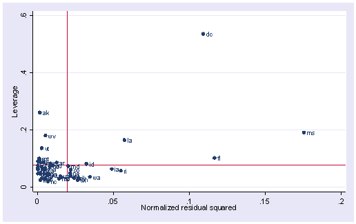
As we have seen, DC is an observation that both has a large residual and large leverage. Such points are potentially the most influential. We can make a plot that shows the leverage by the residual squared and look for observations that are jointly high on both of these measures. We can do this using the lvr2plot command. lvr2plot stands for leverage versus residual squared plot. Using residual squared instead of residual itself, the graph is restricted to the first quadrant and the relative positions of data points are preserved. This is a quick way of checking potential influential observations and outliers at the same time. Both types of points are of great concern for us.
lvr2plot, mlabel(state)
The two reference lines are the means for leverage, horizontal, and for the normalized residual squared, vertical. The points that immediately catch our attention is DC (with the largest leverage) and MS (with the largest residual squared). We’ll look at those observations more carefully by listing them.
list state crime pctmetro poverty single if state=="dc" | state=="ms"

         state     crime   pctmetro    poverty     single
 49.        ms       434       30.7       24.7       14.7
 51.        dc      2922        100       26.4       22.1
Now let’s move on to overall measures of influence, specifically let’s look at Cook’s D and DFITS. These measures both combine information on the residual and leverage. Cook’s D and DFITS are very similar except that they scale differently but they give us similar answers.
The lowest value that Cook’s D can assume is zero, and the higher the Cook’s D is, the more influential the point. The convention cut-off point is 4/n. We can list any observation above the cut-off point by doing the following. We do see that the Cook’s D for DC is by far the largest.
predict d, cooksd
list crime pctmetro poverty single state d if d>4/51

        crime   pctmetro    poverty     single      state          d
  1.      434       30.7       24.7       14.7         ms    .602106
  2.     1062         75       26.4       14.9         la   .1592638
 50.     1206         93       17.8       10.6         fl    .173629
 51.     2922        100       26.4       22.1         dc   3.203429
Now let’s take a look at DFITS. The cut-off point for DFITS is 2*sqrt(k/n). DFITS can be either positive or negative, with numbers close to zero corresponding to the points with small or zero influence. As we see, dfit also indicates that DC is, by far, the most influential observation.
predict dfit, dfits
list crime pctmetro poverty single state dfit if abs(dfit)>2*sqrt(3/51)

        crime   pctmetro    poverty     single      state       dfit
 18.     1206         93       17.8       10.6         fl   .8838196
 49.      434       30.7       24.7       14.7         ms  -1.735096
 50.     1062         75       26.4       14.9         la  -.8181195
 51.     2922        100       26.4       22.1         dc   4.050611
The above measures are general measures of influence. You can also consider more specific measures of influence that assess how each coefficient is changed by deleting the observation. This measure is called DFBETA and is created for each of the predictors. Apparently this is more computational intensive than summary statistics such as Cook’s D since the more predictors a model has, the more computation it may involve. We can restrict our attention to only those predictors that we are most concerned with to see how well behaved those predictors are. In Stata, the dfbeta command will produce the DFBETAs for each of the predictors. The names for the new variables created are chosen by Stata automatically and begin with the letters DF.
dfbeta
                      DFpctmetro:  DFbeta(pctmetro)
                       DFpoverty:  DFbeta(poverty)
                        DFsingle:  DFbeta(single)
This created three variables, DFpctmetro, DFpoverty and DFsingle. Let’s look at the first 5 values.
list state DFpctmetro DFpoverty DFsingle in 1/5

         state  DFpctme~o  DFpoverty   DFsingle
  1.        ak  -.1061846  -.1313398   .1451826
  2.        al   .0124287   .0552852  -.0275128
  3.        ar  -.0687483   .1753482  -.1052626
  4.        az  -.0947614  -.0308833    .001242
  5.        ca   .0126401   .0088009  -.0036361
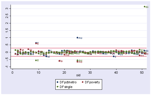
The value for DFsingle for Alaska is .14, which means that by being included in the analysis (as compared to being excluded), Alaska increases the coefficient for single by 0.14 standard errors, i.e., .14 times the standard error for BSingle or by (0.14 * 15.5). Since the inclusion of an observation could either contribute to an increase or decrease in a regression coefficient, DFBETAs can be either positive or negative. A DFBETA value in excess of 2/sqrt(n) merits further investigation. In this example, we would be concerned about absolute values in excess of 2/sqrt(51) or .28.
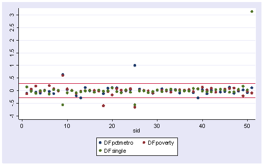
We can plot all three DFBETA values against the state id in one graph shown below. We add a line at .28 and -.28 to help us see potentially troublesome observations. We see the largest value is about 3.0 for DFsingle.
scatter DFpctmetro DFpoverty DFsingle sid, ylabel(-1(.5)3) yline(.28 -.28)
We can repeat this graph with the mlabel() option in the graph command to label the points. With the graph above we can identify which DFBeta is a problem, and with the graph below we can associate that observation with the state that it originates from.
scatter DFpctmetro DFpoverty DFsingle sid, ylabel(-1(.5)3) yline(.28 -.28) ///
  mlabel(state state state)
Now let’s list those observations with DFsingle larger than the cut-off value.
list DFsingle state crime pctmetro poverty single if abs(DFsingle) > 2/sqrt(51)

      DFsingle      state     crime   pctmetro    poverty     single
  9. -.5606022         fl      1206         93       17.8       10.6
 25. -.5680245         ms       434       30.7       24.7       14.7
 51.  3.139084         dc      2922        100       26.4       22.1
The following table summarizes the general rules of thumb we use for these measures to identify observations worthy of further investigation (where k is the number of predictors and n is the number of observations).
| Measure | Value |
| leverage | >(2k+2)/n |
| abs(rstu) | > 2 |
| Cook’s D | > 4/n |
| abs(DFITS) | > 2*sqrt(k/n) |
| abs(DFBETA) | > 2/sqrt(n) |
We have used the predict command to create a number of variables associated with regression analysis and regression diagnostics. The help regress command not only gives help on the regress command, but also lists all of the statistics that can be generated via the predict command. Below we show a snippet of the Stata help file illustrating the various statistics that can be computed via the predict command.
help regress

-------------------------------------------------------------------------------
help for regress                                         (manual:  [R] regress)
-------------------------------------------------------------------------------

<--output omitted-->

The syntax of predict following regress is

        predict [type] newvarname [if exp] [in range] [, statistic]

where statistic is

        xb                           fitted values; the default
        pr(a,b)                      Pr(y |a>y>b)  (a and b may be numbers
        e(a,b)                       E(y |a>y>b)    or variables; a==. means
        ystar(a,b)                   E(y*)          -inf; b==. means inf)
        cooksd                       Cook's distance
        leverage | hat               leverage (diagonal elements of hat matrix)
        residuals                    residuals
        rstandard                    standardized residuals
        rstudent                     Studentized (jackknifed) residuals
        stdp                         standard error of the prediction
        stdf                         standard error of the forecast
        stdr                         standard error of the residual
    (*) covratio                     COVRATIO
    (*) dfbeta(varname)              DFBETA for varname
    (*) dfits                        DFITS
    (*) welsch                       Welsch distance

Unstarred statistics are available both in and out of sample; type "predict ...
if e(sample) ..." if wanted only for the estimation sample.  Starred statistics
are calculated for the estimation sample even when "if e(sample)" is not speci-
fied.

<--more output omitted here.-->
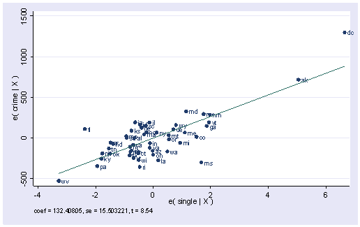
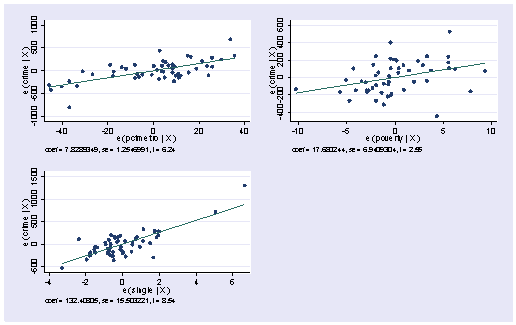
We have explored a number of the statistics that we can get after the regress command. There are also several graphs that can be used to search for unusual and influential observations. The avplot command graphs an added-variable plot. It is also called a partial-regression plot and is very useful in identifying influential points. For example, in the avplot for single shown below, the graph shows crime by single after both crime and single have been adjusted for all other predictors in the model. The line plotted has the same slope as the coefficient for single. This plot shows how the observation for DC influences the coefficient. You can see how the regression line is tugged upwards trying to fit through the extreme value of DC. Alaska and West Virginia may also exert substantial leverage on the coefficient of single.
avplot single, mlabel(state)
Stata also has the avplots command that creates an added variable plot for all of the variables, which can be very useful when you have many variables. It does produce small graphs, but these graphs can quickly reveal whether you have problematic observations based on the added variable plots.
avplots
DC has appeared as an outlier as well as an influential point in every analysis. Since DC is really not a state, we can use this to justify omitting it from the analysis saying that we really wish to just analyze states. First, let’s repeat our analysis including DC by just typing regress.
regress

  Source |       SS       df       MS                  Number of obs =      51
---------+------------------------------               F(  3,    47) =   82.16
   Model |  8170480.21     3  2723493.40               Prob > F      =  0.0000
Residual |  1557994.53    47  33148.8199               R-squared     =  0.8399
---------+------------------------------               Adj R-squared =  0.8296
   Total |  9728474.75    50  194569.495               Root MSE      =  182.07

------------------------------------------------------------------------------
   crime |      Coef.   Std. Err.       t     P>|t|       [95% Conf. Interval]
---------+--------------------------------------------------------------------
pctmetro |   7.828935   1.254699      6.240   0.000       5.304806    10.35306
 poverty |   17.68024    6.94093      2.547   0.014       3.716893    31.64359
  single |   132.4081   15.50322      8.541   0.000       101.2196    163.5965
   _cons |  -1666.436    147.852    -11.271   0.000      -1963.876   -1368.996
------------------------------------------------------------------------------
Now, let’s run the analysis omitting DC by including if state != “dc” on the regress command (here != stands for “not equal to” but you could also use ~= to mean the same thing). As we expect, deleting DC made a large change in the coefficient for single. The coefficient for single dropped from 132.4 to 89.4. After having deleted DC, we would repeat the process we have illustrated in this section to search for any other outlying and influential observations.
regress crime pctmetro poverty single if state!="dc"

  Source |       SS       df       MS                  Number of obs =      50
---------+------------------------------               F(  3,    46) =   39.90
   Model |  3098767.11     3  1032922.37               Prob > F      =  0.0000
Residual |  1190858.11    46  25888.2199               R-squared     =  0.7224
---------+------------------------------               Adj R-squared =  0.7043
   Total |  4289625.22    49  87543.3718               Root MSE      =  160.90

------------------------------------------------------------------------------
   crime |      Coef.   Std. Err.       t     P>|t|       [95% Conf. Interval]
---------+--------------------------------------------------------------------
pctmetro |   7.712334   1.109241      6.953   0.000       5.479547     9.94512
 poverty |   18.28265   6.135958      2.980   0.005       5.931611     30.6337
  single |   89.40078   17.83621      5.012   0.000       53.49836    125.3032
   _cons |  -1197.538   180.4874     -6.635   0.000       -1560.84   -834.2358
------------------------------------------------------------------------------
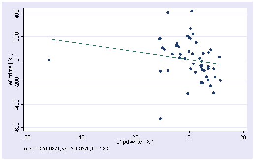
Finally, we showed that the avplot command can be used to searching for outliers among existing variables in your model, but we should note that the avplot command not only works for the variables in the model, it also works for variables that are not in the model, which is why it is called added-variable plot. Let’s use the regression that includes DC as we want to continue to see ill-behavior caused by DC as a demonstration for doing regression diagnostics. We can do an avplot on variable pctwhite.
regress crime pctmetro poverty single
avplot pctwhite
At the top of the plot, we have “coef=-3.509”. It is the coefficient for pctwhite if it were put in the model. We can check that by doing a regression as below.
regress crime pctmetro pctwhite poverty single

  Source |       SS       df       MS                  Number of obs =      51
---------+------------------------------               F(  4,    46) =   63.07
   Model |  8228138.87     4  2057034.72               Prob > F      =  0.0000
Residual |  1500335.87    46  32615.9972               R-squared     =  0.8458
---------+------------------------------               Adj R-squared =  0.8324
   Total |  9728474.75    50  194569.495               Root MSE      =  180.60

------------------------------------------------------------------------------
   crime |      Coef.   Std. Err.       t     P>|t|       [95% Conf. Interval]
---------+--------------------------------------------------------------------
pctmetro |   7.404075   1.284941      5.762   0.000       4.817623    9.990526
pctwhite |  -3.509082   2.639226     -1.330   0.190      -8.821568    1.803404
 poverty |   16.66548   6.927095      2.406   0.020       2.721964      30.609
  single |   120.3576    17.8502      6.743   0.000       84.42702    156.2882
   _cons |  -1191.689   386.0089     -3.087   0.003      -1968.685   -414.6936
------------------------------------------------------------------------------
Summary
In this section, we explored a number of methods of identifying outliers and influential points. In a typical analysis, you would probably use only some of these methods. Generally speaking, there are two types of methods for assessing outliers: statistics such as residuals, leverage, Cook’s D and DFITS, that assess the overall impact of an observation on the regression results, and statistics such as DFBETA that assess the specific impact of an observation on the regression coefficients.
In our example, we found that DC was a point of major concern. We performed a regression with it and without it and the regression equations were very different. We can justify removing it from our analysis by reasoning that our model is to predict crime rate for states, not for metropolitan areas.
2.2 Checking Normality of Residuals
Many researchers believe that multiple regression requires normality. This is not the case. Normality of residuals is only required for valid hypothesis testing, that is, the normality assumption assures that the p-values for the t-tests and F-test will be valid. Normality is not required in order to obtain unbiased estimates of the regression coefficients. OLS regression merely requires that the residuals (errors) be identically and independently distributed. Furthermore, there is no assumption or requirement that the predictor variables be normally distributed. If this were the case than we would not be able to use dummy coded variables in our models.
After we run a regression analysis, we can use the predict command to create residuals and then use commands such as kdensity, qnorm and pnorm to check the normality of the residuals.
Let’s use the elemapi2 data file we saw in Chapter 1 for these analyses. Let’s predict academic performance (api00) from percent receiving free meals (meals), percent of English language learners (ell), and percent of teachers with emergency credentials (emer).
use https://stats.idre.ucla.edu/stat/stata/webbooks/reg/elemapi2
regress api00 meals ell emer

  Source |       SS       df       MS                  Number of obs =     400
---------+------------------------------               F(  3,   396) =  673.00
   Model |  6749782.75     3  2249927.58               Prob > F      =  0.0000
Residual |  1323889.25   396  3343.15467               R-squared     =  0.8360
---------+------------------------------               Adj R-squared =  0.8348
   Total |  8073672.00   399  20234.7669               Root MSE      =   57.82

------------------------------------------------------------------------------
   api00 |      Coef.   Std. Err.       t     P>|t|       [95% Conf. Interval]
---------+--------------------------------------------------------------------
   meals |  -3.159189   .1497371    -21.098   0.000      -3.453568   -2.864809
     ell |  -.9098732   .1846442     -4.928   0.000      -1.272878   -.5468678
    emer |  -1.573496    .293112     -5.368   0.000      -2.149746   -.9972456
   _cons |   886.7033    6.25976    141.651   0.000       874.3967    899.0098
------------------------------------------------------------------------------
We then use the predict command to generate residuals.
predict r, resid
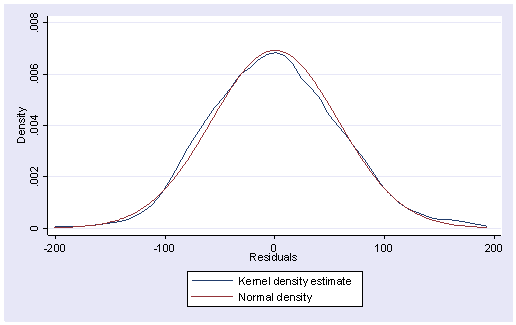
Below we use the kdensity command to produce a kernel density plot with the normal option requesting that a normal density be overlaid on the plot. kdensity stands for kernel density estimate. It can be thought of as a histogram with narrow bins and moving average.
kdensity r, normal
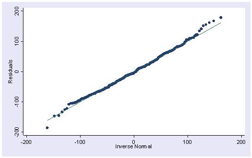
The pnorm command graphs a standardized normal probability (P-P) plot while qnorm plots the quantiles of a variable against the quantiles of a normal distribution. pnorm is sensitive to non-normality in the middle range of data and qnorm is sensitive to non-normality near the tails. As you see below, the results from pnorm show no indications of non-normality, while the qnorm command shows a slight deviation from normal at the upper tail, as can be seen in the kdensity above. Nevertheless, this seems to be a minor and trivial deviation from normality. We can accept that the residuals are close to a normal distribution.
pnorm rqnorm r
There are also numerical tests for testing normality. One of the tests is the test written by Lawrence C. Hamilton, Dept. of Sociology, Univ. of New Hampshire, called iqr. You can get this program from Stata by typing search iqr (see How can I used the search command to search for programs and get additional help? for more information about using search).
iqr stands for inter-quartile range and assumes the symmetry of the distribution. Severe outliers consist of those points that are either 3 inter-quartile-ranges below the first quartile or 3 inter-quartile-ranges above the third quartile. The presence of any severe outliers should be sufficient evidence to reject normality at a 5% significance level. Mild outliers are common in samples of any size. In our case, we don’t have any severe outliers and the distribution seems fairly symmetric. The residuals have an approximately normal distribution.
iqr r

   mean=  7.4e-08         std.dev.=   57.6          (n= 400)
 median= -3.657    pseudo std.dev.=  56.69        (IQR=  76.47)
10 trim= -1.083
                                               low         high
                                               -------------------
                                inner fences   -154.7       151.2
                           # mild outliers     1           5
                           % mild outliers     0.25%       1.25%

                                outer fences   -269.4       265.9
                           # severe outliers   0           0
                           % severe outliers   0.00%       0.00%
Another test available is the swilk test which performs the Shapiro-Wilk W test for normality. The p-value is based on the assumption that the distribution is normal. In our example, it is very large (.51), indicating that we cannot reject that r is normally distributed.
swilk r

                   Shapiro-Wilk W test for normal data
 Variable |    Obs           W         V          z   Pr > z
 ---------+-------------------------------------------------
        r |    400     0.99641     0.989     -0.025  0.51006
2.3 Checking Homoscedasticity of Residuals
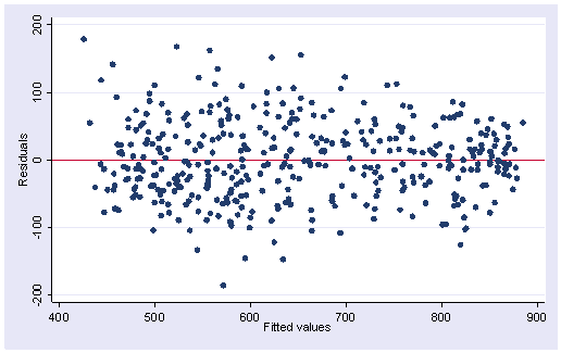
One of the main assumptions for the ordinary least squares regression is the homogeneity of variance of the residuals. If the model is well-fitted, there should be no pattern to the residuals plotted against the fitted values. If the variance of the residuals is non-constant then the residual variance is said to be “heteroscedastic.” There are graphical and non-graphical methods for detecting heteroscedasticity. A commonly used graphical method is to plot the residuals versus fitted (predicted) values. We do this by issuing the rvfplot command. Below we use the rvfplot command with the yline(0) option to put a reference line at y=0. We see that the pattern of the data points is getting a little narrower towards the right end, which is an indication of heteroscedasticity.
rvfplot, yline(0)
Now let’s look at a couple of commands that test for heteroscedasticity.
estat imtest

Cameron & Trivedi's decomposition of IM-test

---------------------------------------------------
              Source |       chi2     df      p
---------------------+-----------------------------
  Heteroskedasticity |      18.35      9    0.0313
            Skewness |       7.78      3    0.0507
            Kurtosis |       0.27      1    0.6067
---------------------+-----------------------------
               Total |      26.40     13    0.0150
---------------------------------------------------
estat hettestBreusch-Pagan / Cook-Weisberg test for heteroskedasticity Ho: Constant variance Variables: fitted values of api00chi2(1) = 8.75 Prob > chi2 = 0.0031
The first test on heteroskedasticity given by imest is the White’s test and the second one given by hettest is the Breusch-Pagan test. Both test the null hypothesis that the variance of the residuals is homogenous. Therefore, if the p-value is very small, we would have to reject the hypothesis and accept the alternative hypothesis that the variance is not homogenous. So in this case, the evidence is against the null hypothesis that the variance is homogeneous. These tests are very sensitive to model assumptions, such as the assumption of normality. Therefore it is a common practice to combine the tests with diagnostic plots to make a judgment on the severity of the heteroscedasticity and to decide if any correction is needed for heteroscedasticity. In our case, the plot above does not show too strong an evidence. So we are not going to get into details on how to correct for heteroscedasticity even though there are methods available.
2.4 Checking for Multicollinearity
When there is a perfect linear relationship among the predictors, the estimates for a regression model cannot be uniquely computed. The term collinearity implies that two variables are near perfect linear combinations of one another. When more than two variables are involved it is often called multicollinearity, although the two terms are often used interchangeably.
The primary concern is that as the degree of multicollinearity increases, the regression model estimates of the coefficients become unstable and the standard errors for the coefficients can get wildly inflated. In this section, we will explore some Stata commands that help to detect multicollinearity.
We can use the vif command after the regression to check for multicollinearity. vif stands for variance inflation factor. As a rule of thumb, a variable whose VIF values are greater than 10 may merit further investigation. Tolerance, defined as 1/VIF, is used by many researchers to check on the degree of collinearity. A tolerance value lower than 0.1 is comparable to a VIF of 10. It means that the variable could be considered as a linear combination of other independent variables. Let’s first look at the regression we did from the last section, the regression model predicting api00 from meals, ell and emer and then issue the vif command.
regress api00 meals ell emer

<-- output omitted -->

vif

Variable |      VIF      1/VIF
---------+----------------------
   meals |      2.73    0.366965
     ell |      2.51    0.398325
    emer |      1.41    0.706805
---------+----------------------
Mean VIF |      2.22
The VIFs look fine here. Here is an example where the VIFs are more worrisome.
regress api00 acs_k3 avg_ed grad_sch col_grad some_col

  Source |       SS       df       MS                  Number of obs =     379
---------+------------------------------               F(  5,   373) =  143.79
   Model |  5056268.54     5  1011253.71               Prob > F      =  0.0000
Residual |  2623191.21   373  7032.68421               R-squared     =  0.6584
---------+------------------------------               Adj R-squared =  0.6538
   Total |  7679459.75   378  20316.0311               Root MSE      =  83.861

------------------------------------------------------------------------------
   api00 |      Coef.   Std. Err.       t     P>|t|       [95% Conf. Interval]
---------+--------------------------------------------------------------------
  acs_k3 |   11.45725   3.275411      3.498   0.001        5.01667    17.89784
  avg_ed |   227.2638    37.2196      6.106   0.000       154.0773    300.4504
grad_sch |  -2.090898   1.352292     -1.546   0.123      -4.749969    .5681734
col_grad |  -2.967831   1.017812     -2.916   0.004      -4.969199   -.9664627
some_col |  -.7604543   .8109676     -0.938   0.349      -2.355096    .8341871
   _cons |  -82.60913   81.84638     -1.009   0.313      -243.5473    78.32903
------------------------------------------------------------------------------

vif

Variable |      VIF      1/VIF
---------+----------------------
  avg_ed |     43.57    0.022951
grad_sch |     14.86    0.067274
col_grad |     14.78    0.067664
some_col |      4.07    0.245993
  acs_k3 |      1.03    0.971867
---------+----------------------
Mean VIF |     15.66
In this example, the VIF and tolerance (1/VIF) values for avg_ed grad_sch and col_grad are worrisome. All of these variables measure education of the parents and the very high VIF values indicate that these variables are possibly redundant. For example, after you know grad_sch and col_grad, you probably can predict avg_ed very well. In this example, multicollinearity arises because we have put in too many variables that measure the same thing, parent education.
Let’s omit one of the parent education variables, avg_ed. Note that the VIF values in the analysis below appear much better. Also, note how the standard errors are reduced for the parent education variables, grad_sch and col_grad. This is because the high degree of collinearity caused the standard errors to be inflated. With the multicollinearity eliminated, the coefficient for grad_sch, which had been non-significant, is now significant.
regress api00 acs_k3 grad_sch col_grad some_col

  Source |       SS       df       MS                  Number of obs =     398
---------+------------------------------               F(  4,   393) =  107.12
   Model |  4180144.34     4  1045036.09               Prob > F      =  0.0000
Residual |  3834062.79   393  9755.88497               R-squared     =  0.5216
---------+------------------------------               Adj R-squared =  0.5167
   Total |  8014207.14   397  20186.9197               Root MSE      =  98.772

------------------------------------------------------------------------------
   api00 |      Coef.   Std. Err.       t     P>|t|       [95% Conf. Interval]
---------+--------------------------------------------------------------------
  acs_k3 |    11.7126   3.664872      3.196   0.002       4.507392    18.91781
grad_sch |   5.634762   .4581979     12.298   0.000       4.733937    6.535588
col_grad |   2.479916   .3395548      7.303   0.000       1.812345    3.147487
some_col |   2.158271   .4438822      4.862   0.000        1.28559    3.030952
   _cons |   283.7446   70.32475      4.035   0.000       145.4849    422.0044
------------------------------------------------------------------------------

vif

Variable |      VIF      1/VIF
---------+----------------------
col_grad |      1.28    0.782726
grad_sch |      1.26    0.792131
some_col |      1.03    0.966696
  acs_k3 |      1.02    0.976666
---------+----------------------
Mean VIF |      1.15
Let’s introduce another command on collinearity. The collin command displays several different measures of collinearity. For example, we can test for collinearity among the variables we used in the two examples above. Note that the collin command does not need to be run in connection with a regress command, unlike the vif command which follows a regress command. Also note that only predictor (independent) variables are used with the collin command. You can download collin from within Stata by typing search collin (see How can I used the search command to search for programs and get additional help? for more information about using search).
collin acs_k3  avg_ed grad_sch col_grad some_col

  Collinearity Diagnostics

                        SQRT                           Cond
  Variable       VIF    VIF    Tolerance  Eigenval     Index
-------------------------------------------------------------
    acs_k3      1.03    1.01    0.9719     2.4135     1.0000
    avg_ed     43.57    6.60    0.0230     1.0917     1.4869
  grad_sch     14.86    3.86    0.0673     0.9261     1.6144
  col_grad     14.78    3.84    0.0677     0.5552     2.0850
  some_col      4.07    2.02    0.2460     0.0135    13.3729
-------------------------------------------------------------
  Mean VIF     15.66              Condition Number   13.3729
We now remove avg_ed and see the collinearity diagnostics improve considerably.
collin acs_k3 grad_sch col_grad some_col

  Collinearity Diagnostics

                        SQRT                           Cond
  Variable       VIF    VIF    Tolerance  Eigenval     Index
-------------------------------------------------------------
    acs_k3      1.02    1.01    0.9767     1.5095     1.0000
  grad_sch      1.26    1.12    0.7921     1.0407     1.2043
  col_grad      1.28    1.13    0.7827     0.9203     1.2807
  some_col      1.03    1.02    0.9667     0.5296     1.6883
-------------------------------------------------------------
  Mean VIF      1.15              Condition Number    1.6883
The condition number is a commonly used index of the global instability of the regression coefficients — a large condition number, 10 or more, is an indication of instability.
2.5 Checking Linearity
When we do linear regression, we assume that the relationship between the response variable and the predictors is linear. This is the assumption of linearity. If this assumption is violated, the linear regression will try to fit a straight line to data that does not follow a straight line. Checking the linear assumption in the case of simple regression is straightforward, since we only have one predictor. All we have to do is a scatter plot between the response variable and the predictor to see if nonlinearity is present, such as a curved band or a big wave-shaped curve. For example, recall we did a simple linear regression in Chapter 1 using dataset elemapi2.
use https://stats.idre.ucla.edu/stat/stata/webbooks/reg/elemapi2
regress api00 enroll

  Source |       SS       df       MS                  Number of obs =     400
---------+------------------------------               F(  1,   398) =   44.83
   Model |  817326.293     1  817326.293               Prob > F      =  0.0000
Residual |  7256345.70   398  18232.0244               R-squared     =  0.1012
---------+------------------------------               Adj R-squared =  0.0990
   Total |  8073672.00   399  20234.7669               Root MSE      =  135.03

------------------------------------------------------------------------------
   api00 |      Coef.   Std. Err.       t     P>|t|       [95% Conf. Interval]
---------+--------------------------------------------------------------------
  enroll |  -.1998674   .0298512     -6.695   0.000      -.2585532   -.1411817
   _cons |   744.2514   15.93308     46.711   0.000       712.9279    775.5749
------------------------------------------------------------------------------
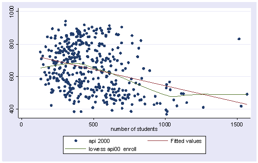
Below we use the scatter command to show a scatterplot predicting api00 from enroll and use lfit to show a linear fit, and then lowess to show a lowess smoother predicting api00 from enroll. We clearly see some degree of nonlinearity.
twoway (scatter api00 enroll) (lfit api00 enroll) (lowess api00 enroll)
Checking the linearity assumption is not so straightforward in the case of multiple regression. We will try to illustrate some of the techniques that you can use. The most straightforward thing to do is to plot the standardized residuals against each of the predictor variables in the regression model. If there is a clear nonlinear pattern, there is a problem of nonlinearity. Otherwise, we should see for each of the plots just a random scatter of points. Let’s continue to use dataset elemapi2 here. Let’s use a different model.
regress api00 meals some_col Source | SS df MS Number of obs = 400 ---------+------------------------------ F( 2, 397) = 877.98 Model | 6584905.75 2 3292452.87 Prob > F = 0.0000 Residual | 1488766.25 397 3750.04094 R-squared = 0.8156 ---------+------------------------------ Adj R-squared = 0.8147 Total | 8073672.00 399 20234.7669 Root MSE = 61.238 ------------------------------------------------------------------------------ api00 | Coef. Std. Err. t P>|t| [95% Conf. Interval] ---------+-------------------------------------------------------------------- meals | -3.949 .0984576 -40.109 0.000 -4.142563 -3.755436 some_col | .8476549 .2771428 3.059 0.002 .302804 1.392506 _cons | 869.097 9.417734 92.283 0.000 850.5822 887.6119 ------------------------------------------------------------------------------ predict r, resid scatter r mealsscatter r some_col
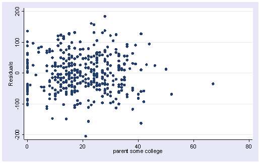
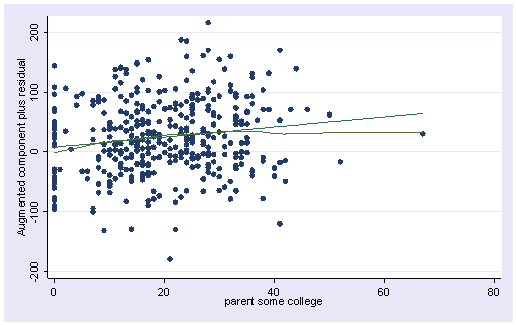
The two residual versus predictor variable plots above do not indicate strongly a clear departure from linearity. Another command for detecting non-linearity is acprplot. acprplot graphs an augmented component-plus-residual plot, a.k.a. augmented partial residual plot. It can be used to identify nonlinearities in the data. Let’s use the acprplot command for meals and some_col and use the lowess lsopts(bwidth(1)) options to request lowess smoothing with a bandwidth of 1.
In the first plot below the smoothed line is very close to the ordinary regression line, and the entire pattern seems pretty uniform. The second plot does seem more problematic at the right end. This may come from some potential influential points. Overall, they don’t look too bad and we shouldn’t be too concerned about non-linearities in the data.
acprplot meals, lowess lsopts(bwidth(1))acprplot some_col, lowess lsopts(bwidth(1))
We have seen how to use acprplot to detect nonlinearity. However our last example didn’t show much nonlinearity. Let’s look at a more interesting example. This example is taken from “Statistics with Stata 5” by Lawrence C. Hamilton (1997, Duxbery Press). The dataset we will use is called nations.dta. We can get the dataset from the Internet.
use https://stats.idre.ucla.edu/stat/stata/examples/sws5/nations
(Data on 109 countries)

describe

Contains data from https://stats.idre.ucla.edu/stat/stata/examples/sws5/nations.dta
  obs:           109                          Data on 109 countries
 vars:            15                          22 Dec 1996 20:12
 size:         4,033 (98.3% of memory free)
-------------------------------------------------------------------------------
   1. country   str8   %9s                    Country
   2. pop       float  %9.0g                  1985 population in millions
   3. birth     byte   %8.0g                  Crude birth rate/1000 people
   4. death     byte   %8.0g                  Crude death rate/1000 people
   5. chldmort  byte   %8.0g                  Child (1-4 yr) mortality 1985
   6. infmort   int    %8.0g                  Infant (<1 yr) mortality 1985
   7. life      byte   %8.0g                  Life expectancy at birth 1985
   8. food      int    %8.0g                  Per capita daily calories 1985
   9. energy    int    %8.0g                  Per cap energy consumed, kg oil
  10. gnpcap    int    %8.0g                  Per capita GNP 1985
  11. gnpgro    float  %9.0g                  Annual GNP growth % 65-85
  12. urban     byte   %8.0g                  % population urban 1985
  13. school1   int    %8.0g                  Primary enrollment % age-group
  14. school2   byte   %8.0g                  Secondary enroll % age-group
  15. school3   byte   %8.0g                  Higher ed. enroll % age-group
-------------------------------------------------------------------------------
Sorted by:
Let’s build a model that predicts birth rate (birth), from per capita gross national product (gnpcap), and urban population (urban). If this were a complete regression analysis, we would start with examining the variables, but for the purpose of illustrating nonlinearity, we will jump directly to the regression.
regress birth gnpcap urban
  Source |       SS       df       MS                  Number of obs =     108
---------+------------------------------               F(  2,   105) =   64.22
   Model |   10796.488     2  5398.24399               Prob > F      =  0.0000
Residual |   8825.5861   105   84.053201               R-squared     =  0.5502
---------+------------------------------               Adj R-squared =  0.5417
   Total |  19622.0741   107   183.38387               Root MSE      =  9.1681

------------------------------------------------------------------------------
   birth |      Coef.   Std. Err.       t     P>|t|       [95% Conf. Interval]
---------+--------------------------------------------------------------------
  gnpcap |   -.000842   .0002637     -3.193   0.002      -.0013649   -.0003191
   urban |  -.2823184   .0462191     -6.108   0.000      -.3739624   -.1906744
   _cons |   48.85603   1.986909     24.589   0.000       44.91635     52.7957
------------------------------------------------------------------------------
Now, let’s do the acprplot on our predictors.
acprplot gnpcap, lowess
acprplot urban, lowess
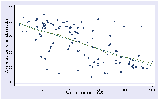
The acprplot plot for gnpcap shows clear deviation from linearity and the one for urban does not show nearly as much deviation from linearity. Now, let’s look at these variables more closely.
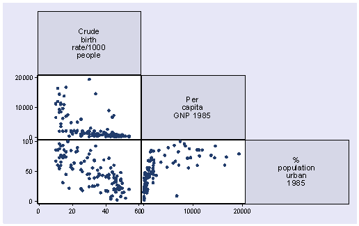
graph matrix birth gnpcap urban, half
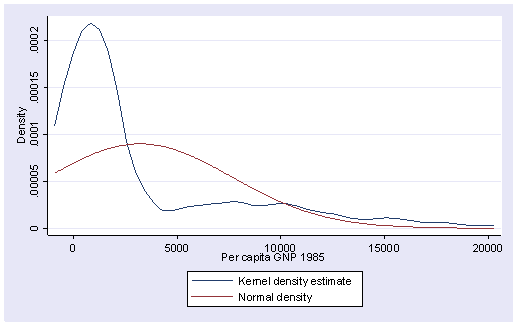
We see that the relation between birth rate and per capita gross national product is clearly nonlinear and the relation between birth rate and urban population is not too far off from being linear. So let’s focus on variable gnpcap. First let’s look at the distribution of gnpcap. We suspect that gnpcap may be very skewed. This may affect the appearance of the acprplot.
kdensity gnpcap, normal
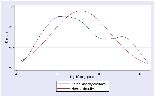
Indeed, it is very skewed. This suggests to us that some transformation of the variable may be necessary. One of the commonly used transformations is log transformation. Let’s try it here.
generate lggnp=log(gnpcap)
label variable lggnp "log-10 of gnpcap"
kdensity lggnp, normal
The transformation does seem to help correct the skewness greatly. Next, let’s do the regression again replacing gnpcap by lggnp.
regress birth lggnp urban

  Source |       SS       df       MS                  Number of obs =     108
---------+------------------------------               F(  2,   105) =   76.20
   Model |  11618.0395     2  5809.01974               Prob > F      =  0.0000
Residual |   8004.0346   105  76.2289009               R-squared     =  0.5921
---------+------------------------------               Adj R-squared =  0.5843
   Total |  19622.0741   107   183.38387               Root MSE      =  8.7309

------------------------------------------------------------------------------
   birth |      Coef.   Std. Err.       t     P>|t|       [95% Conf. Interval]
---------+--------------------------------------------------------------------
   lggnp |  -4.877688   1.039477     -4.692   0.000       -6.93878   -2.816596
   urban |   -.156254   .0579632     -2.696   0.008      -.2711843   -.0413237
   _cons |   74.87778   5.439654     13.765   0.000       64.09196    85.66361
------------------------------------------------------------------------------

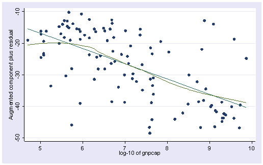
acprplot lggnp, lowess
The plot above shows less deviation from nonlinearity than before, though the problem of nonlinearity has not been completely solved yet.
2.6 Model Specification
A model specification error can occur when one or more relevant variables are omitted from the model or one or more irrelevant variables are included in the model. If relevant variables are omitted from the model, the common variance they share with included variables may be wrongly attributed to those variables, and the error term is inflated. On the other hand, if irrelevant variables are included in the model, the common variance they share with included variables may be wrongly attributed to them. Model specification errors can substantially affect the estimate of regression coefficients.
Consider the model below. This regression suggests that as class size increases the academic performance increases. Before we publish results saying that increased class size is associated with higher academic performance, let’s check the model specification.
use https://stats.idre.ucla.edu/stat/stata/webbooks/reg/elemapi2

regress api00  acs_k3

      Source |       SS       df       MS              Number of obs =     398
-------------+------------------------------           F(  1,   396) =   11.93
       Model |  234353.831     1  234353.831           Prob > F      =  0.0006
    Residual |  7779853.31   396  19646.0942           R-squared     =  0.0292
-------------+------------------------------           Adj R-squared =  0.0268
       Total |  8014207.14   397  20186.9197           Root MSE      =  140.16

------------------------------------------------------------------------------
       api00 |      Coef.   Std. Err.      t    P>|t|     [95% Conf. Interval]
-------------+----------------------------------------------------------------
      acs_k3 |   17.75148   5.139688     3.45   0.001     7.646998    27.85597
       _cons |   308.3372   98.73085     3.12   0.002      114.235    502.4393
------------------------------------------------------------------------------
There are a couple of methods to detect specification errors. The linktest command performs a model specification link test for single-equation models. linktest is based on the idea that if a regression is properly specified, one should not be able to find any additional independent variables that are significant except by chance. linktest creates two new variables, the variable of prediction, _hat, and the variable of squared prediction, _hatsq. The model is then refit using these two variables as predictors. _hat should be significant since it is the predicted value. On the other hand, _hatsq shouldn’t, because if our model is specified correctly, the squared predictions should not have much explanatory power. That is we wouldn’t expect _hatsq to be a significant predictor if our model is specified correctly. So we will be looking at the p-value for _hatsq.
linktest

      Source |       SS       df       MS              Number of obs =     398
-------------+------------------------------           F(  2,   395) =    7.09
       Model |  277705.911     2  138852.955           Prob > F      =  0.0009
    Residual |  7736501.23   395  19586.0791           R-squared     =  0.0347
-------------+------------------------------           Adj R-squared =  0.0298
       Total |  8014207.14   397  20186.9197           Root MSE      =  139.95

------------------------------------------------------------------------------
       api00 |      Coef.   Std. Err.      t    P>|t|     [95% Conf. Interval]
-------------+----------------------------------------------------------------
        _hat |  -11.05006   8.104639    -1.36   0.174    -26.98368    4.883562
      _hatsq |   .0093318   .0062724     1.49   0.138    -.0029996    .0216631
       _cons |    3884.48   2617.695     1.48   0.139    -1261.877    9030.837
------------------------------------------------------------------------------
From the above linktest, the test of _hatsq is not significant. This is to say that linktest has failed to reject the assumption that the model is specified correctly. Therefore, it seems to us that we don’t have a specification error. But now, let’s look at another test before we jump to the conclusion.
The ovtest command performs another test of regression model specification. It performs a regression specification error test (RESET) for omitted variables. The idea behind ovtest is very similar to linktest. It also creates new variables based on the predictors and refits the model using those new variables to see if any of them would be significant. Let’s try ovtest on our model.
ovtest

Ramsey RESET test using powers of the fitted values of api00
       Ho:  model has no omitted variables
                 F(3, 393) =      4.13
                  Prob > F =      0.0067
The ovtest command indicates that there are omitted variables. So we have tried both the linktest and ovtest, and one of them (ovtest) tells us that we have a specification error. We therefore have to reconsider our model.
Let’s try adding the variable full to the model. Now, both the linktest and ovtest are significant, indicating we have a specification error.
regress api00 acs_k3 full

      Source |       SS       df       MS              Number of obs =     398
-------------+------------------------------           F(  2,   395) =  101.19
       Model |  2715101.89     2  1357550.95           Prob > F      =  0.0000
    Residual |  5299105.24   395  13415.4563           R-squared     =  0.3388
-------------+------------------------------           Adj R-squared =  0.3354
       Total |  8014207.14   397  20186.9197           Root MSE      =  115.83

------------------------------------------------------------------------------
       api00 |      Coef.   Std. Err.      t    P>|t|     [95% Conf. Interval]
-------------+----------------------------------------------------------------
      acs_k3 |   8.355681   4.303023     1.94   0.053    -.1040088    16.81537
        full |   5.389788   .3963539    13.60   0.000     4.610561    6.169015
       _cons |   32.21346   84.07525     0.38   0.702    -133.0775    197.5044
------------------------------------------------------------------------------

linktest

      Source |       SS       df       MS              Number of obs =     398
-------------+------------------------------           F(  2,   395) =  108.32
       Model |  2838564.40     2  1419282.20           Prob > F      =  0.0000
    Residual |  5175642.74   395   13102.893           R-squared     =  0.3542
-------------+------------------------------           Adj R-squared =  0.3509
       Total |  8014207.14   397  20186.9197           Root MSE      =  114.47

------------------------------------------------------------------------------
       api00 |      Coef.   Std. Err.      t    P>|t|     [95% Conf. Interval]
-------------+----------------------------------------------------------------
        _hat |  -1.868895   .9371889    -1.99   0.047    -3.711397   -.0263936
      _hatsq |   .0023436   .0007635     3.07   0.002     .0008426    .0038447
       _cons |   858.8726   283.4594     3.03   0.003     301.5948     1416.15
------------------------------------------------------------------------------

ovtest

Ramsey RESET test using powers of the fitted values of api00
       Ho:  model has no omitted variables
                 F(3, 392) =      4.09
                  Prob > F =      0.0071
Let’s try adding one more variable, meals, to the above model.
regress api00  acs_k3 full meals

      Source |       SS       df       MS              Number of obs =     398
-------------+------------------------------           F(  3,   394) =  615.55
       Model |  6604966.18     3  2201655.39           Prob > F      =  0.0000
    Residual |  1409240.96   394   3576.7537           R-squared     =  0.8242
-------------+------------------------------           Adj R-squared =  0.8228
       Total |  8014207.14   397  20186.9197           Root MSE      =  59.806

------------------------------------------------------------------------------
       api00 |      Coef.   Std. Err.      t    P>|t|     [95% Conf. Interval]
-------------+----------------------------------------------------------------
      acs_k3 |  -.7170622   2.238821    -0.32   0.749    -5.118592    3.684468
        full |   1.327138   .2388739     5.56   0.000      .857511    1.796765
       meals |  -3.686265   .1117799   -32.98   0.000    -3.906024   -3.466505
       _cons |   771.6581   48.86071    15.79   0.000     675.5978    867.7184
------------------------------------------------------------------------------

linktest

      Source |       SS       df       MS              Number of obs =     398
-------------+------------------------------           F(  2,   395) =  931.68
       Model |  6612479.76     2  3306239.88           Prob > F      =  0.0000
    Residual |  1401727.38   395  3548.67691           R-squared     =  0.8251
-------------+------------------------------           Adj R-squared =  0.8242
       Total |  8014207.14   397  20186.9197           Root MSE      =  59.571

------------------------------------------------------------------------------
       api00 |      Coef.   Std. Err.      t    P>|t|     [95% Conf. Interval]
-------------+----------------------------------------------------------------
        _hat |    1.42433   .2925374     4.87   0.000      .849205    1.999455
      _hatsq |  -.0003172    .000218    -1.46   0.146    -.0007458    .0001114
       _cons |  -136.5102   95.05904    -1.44   0.152    -323.3951     50.3747
------------------------------------------------------------------------------

ovtest

Ramsey RESET test using powers of the fitted values of api00
       Ho:  model has no omitted variables
                 F(3, 391) =      2.56
                  Prob > F =      0.0545
The linktest is once again non-significant while the p-value for ovtest is slightly greater than .05. Note that after including meals and full, the coefficient for class size is no longer significant. While acs_k3 does have a positive relationship with api00 when no other variables are in the model, when we include, and hence control for, other important variables, acs_k3 is no longer significantly related to api00 and its relationship to api00 is no longer positive.
linktest and ovtest are tools available in Stata for checking specification errors, though linktest can actually do more than check omitted variables as we used here, e.g., checking the correctness of link function specification. For more details on those tests, please refer to Stata manual.
2.7 Issues of Independence
The statement of this assumption that the errors associated with one observation are not correlated with the errors of any other observation cover several different situations. Consider the case of collecting data from students in eight different elementary schools. It is likely that the students within each school will tend to be more like one another than students from different schools, that is, their errors are not independent. We will deal with this type of situation in Chapter 4 when we demonstrate the regress command with cluster option.
Another way in which the assumption of independence can be broken is when data are collected on the same variables over time. Let’s say that we collect truancy data every semester for 12 years. In this situation it is likely that the errors for observation between adjacent semesters will be more highly correlated than for observations more separated in time. This is known as autocorrelation. When you have data that can be considered to be time-series you should use the dwstat command that performs a Durbin-Watson test for correlated residuals.
We don’t have any time-series data, so we will use the elemapi2 dataset and pretend that snum indicates the time at which the data were collected. We will also need to use the tsset command to let Stata know which variable is the time variable.
use https://stats.idre.ucla.edu/stat/stata/webbooks/reg/elemapi2
tsset snum
        time variable:  snum, 58 to 6072, but with gaps

regress api00 enroll

( output omitted )

dwstat

Number of gaps in sample:  311
Durbin-Watson d-statistic(  2,   400) =  .2892712
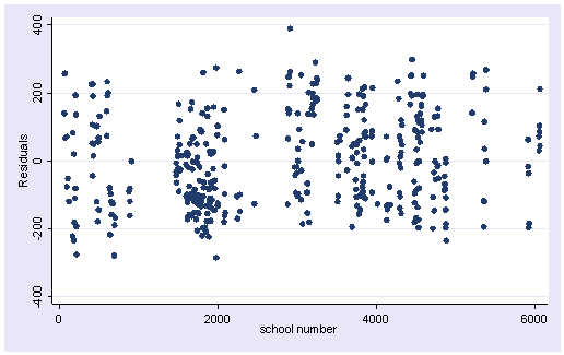
The Durbin-Watson statistic has a range from 0 to 4 with a midpoint of 2. The observed value in our example is very small, close to zero, which is not surprising since our data are not truly time-series. A simple visual check would be to plot the residuals versus the time variable.
. predict r, resid

scatter r snum
2.8 Summary
In this chapter, we have used a number of tools in Stata for determining whether our data meets the regression assumptions. Below, we list the major commands we demonstrated organized according to the assumption the command was shown to test.
- Detecting Unusual and Influential Data
- predict — used to create predicted values, residuals, and measures of influence.
- rvpplot — graphs a residual-versus-predictor plot.
- rvfplot — graphs residual-versus-fitted plot.
- lvr2plot — graphs a leverage-versus-squared-residual plot.
- dfbeta — calculates DFBETAs for all the independent variables in the linear model.
- avplot — graphs an added-variable plot, a.k.a. partial regression plot.
- Tests for Normality of Residuals
- kdensity — produces kernel density plot with normal distribution overlayed.
- pnorm — graphs a standardized normal probability (P-P) plot.
- qnorm — plots the quantiles of varname against the quantiles of a normal distribution.
- iqr — resistant normality check and outlier identification.
- swilk — performs the Shapiro-Wilk W test for normality.
- Tests for Heteroscedasticity
- rvfplot — graphs residual-versus-fitted plot.
- hettest — performs Cook and Weisberg test for heteroscedasticity.
- whitetst — computes the White general test for Heteroscedasticity.
- Tests for Multicollinearity
- vif — calculates the variance inflation factor for the independent variables in the linear model.
- collin — calculates the variance inflation factor and other multicollinearity diagnostics
- Tests for Non-Linearity
- acprplot — graphs an augmented component-plus-residual plot.
- cprplot — graphs component-plus-residual plot, a.k.a. residual plot.
- Tests for Model Specification
- linktest — performs a link test for model specification.
- ovtest — performs regression specification error test (RESET) for omitted variables.
2.9 Self Assessment
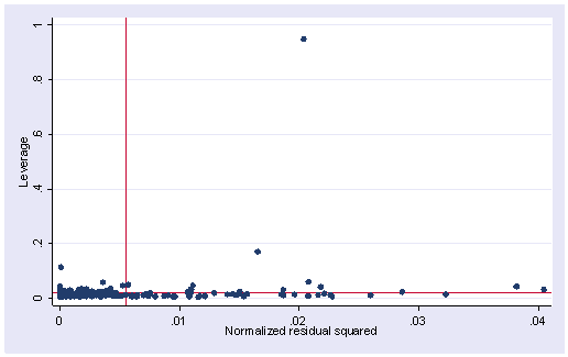
1. The following data set consists of measured weight, measured height, reported weight and reported height of some 200 people. You can get it from within Stata by typing use https://stats.idre.ucla.edu/stat/stata/webbooks/reg/davis We tried to build a model to predict measured weight by reported weight, reported height and measured height. We did an lvr2plot after the regression and here is what we have. Explain what you see in the graph and try to use other STATA commands to identify the problematic observation(s). What do you think the problem is and what is your solution?
use https://stats.idre.ucla.edu/stat/stata/webbooks/reg/davis
. regress  measwt measht reptwt reptht
  Source |       SS       df       MS                  Number of obs =     181
---------+------------------------------               F(  3,   177) = 1640.88
   Model |  40891.9594     3  13630.6531               Prob > F      =  0.0000
Residual |   1470.3279   177  8.30693727               R-squared     =  0.9653
---------+------------------------------               Adj R-squared =  0.9647
   Total |  42362.2873   180  235.346041               Root MSE      =  2.8822

------------------------------------------------------------------------------
  measwt |      Coef.   Std. Err.       t     P>|t|       [95% Conf. Interval]
---------+--------------------------------------------------------------------
  measht |  -.9607757   .0260189    -36.926   0.000      -1.012123   -.9094285
  reptwt |    1.01917   .0240778     42.328   0.000        .971654    1.066687
  reptht |   .8184156   .0419658     19.502   0.000       .7355979    .9012334
   _cons |    24.8138   4.888302      5.076   0.000       15.16695    34.46065
------------------------------------------------------------------------------
lvr2plot
2. Using the data from the last exercise, what measure would you use if you want to know how much change an observation would make on a coefficient for a predictor? For example, show how much change would it be for the coefficient of predictor reptht if we omit observation 12 from our regression analysis? What are the other measures that you would use to assess the influence of an observation on regression? What are the cut-off values for them?
3. The following data file is called bbwt.dta and it is from Weisberg’s Applied Regression Analysis. You can obtain it from within Stata by typing use https://stats.idre.ucla.edu/stat/stata/webbooks/reg/bbwt It consists of the body weights and brain weights of some 60 animals. We want to predict the brain weight by body weight, that is, a simple linear regression of brain weight against body weight. Show what you have to do to verify the linearity assumption. If you think that it violates the linearity assumption, show some possible remedies that you would consider.
use https://stats.idre.ucla.edu/stat/stata/webbooks/reg/bbwt, clear
regress brainwt bodywt
Source | SS df MS Number of obs = 62 ---------+------------------------------ F( 1, 60) = 411.12 Model | 46067326.8 1 46067326.8 Prob > F = 0.0000 Residual | 6723217.18 60 112053.62 R-squared = 0.8726 ---------+------------------------------ Adj R-squared = 0.8705 Total | 52790543.9 61 865418.753 Root MSE = 334.74 ------------------------------------------------------------------------------ brainwt | Coef. Std. Err. t P>|t| [95% Conf. Interval] ---------+-------------------------------------------------------------------- bodywt | .9664599 .0476651 20.276 0.000 .8711155 1.061804 _cons | 91.00865 43.55574 2.089 0.041 3.884201 178.1331 ------------------------------------------------------------------------------
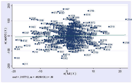
4. We did a regression analysis using the data file elemapi2 in chapter 2. Continuing with the analysis we did, we did an avplot here. Explain what an avplot is and what type of information you would get from the plot. If variable full were put in the model, would it be a significant predictor?
use https://stats.idre.ucla.edu/stat/stata/webbooks/reg/elemapi2, clear
regress api00 meals ell emer
Source | SS df MS Number of obs = 400 ---------+------------------------------ F( 3, 396) = 673.00 Model | 6749782.75 3 2249927.58 Prob > F = 0.0000 Residual | 1323889.25 396 3343.15467 R-squared = 0.8360 ---------+------------------------------ Adj R-squared = 0.8348 Total | 8073672.00 399 20234.7669 Root MSE = 57.82 ------------------------------------------------------------------------------ api00 | Coef. Std. Err. t P>|t| [95% Conf. Interval] ---------+-------------------------------------------------------------------- meals | -3.159189 .1497371 -21.098 0.000 -3.453568 -2.864809 ell | -.9098732 .1846442 -4.928 0.000 -1.272878 -.5468678 emer | -1.573496 .293112 -5.368 0.000 -2.149746 -.9972456 _cons | 886.7033 6.25976 141.651 0.000 874.3967 899.0098 ------------------------------------------------------------------------------avplot full, mlabel(snum)
5. The data set wage.dta is from a national sample of 6000 households with a male head earning less than $15,000 annually in 1966. You can get this data file by typing use https://stats.idre.ucla.edu/stat/stata/webbooks/reg/wage from within Stata. The data were classified into 39 demographic groups for analysis. We tried to predict the average hours worked by average age of respondent and average yearly non-earned income.
use https://stats.idre.ucla.edu/stat/stata/webbooks/reg/wage, clear. regress HRS AGE NEINSource | SS df MS Number of obs = 39 ---------+------------------------------ F( 2, 36) = 39.72 Model | 107205.109 2 53602.5543 Prob > F = 0.0000 Residual | 48578.1222 36 1349.39228 R-squared = 0.6882 ---------+------------------------------ Adj R-squared = 0.6708 Total | 155783.231 38 4099.5587 Root MSE = 36.734 ------------------------------------------------------------------------------ HRS | Coef. Std. Err. t P>|t| [95% Conf. Interval] ---------+-------------------------------------------------------------------- AGE | -8.281632 1.603736 -5.164 0.000 -11.53416 -5.029104 NEIN | .4289202 .0484882 8.846 0.000 .3305816 .5272588 _cons | 2321.03 57.55038 40.330 0.000 2204.312 2437.748 ------------------------------------------------------------------------------
Both predictors are significant. Now if we add ASSET to our predictors list, neither NEIN nor ASSET is significant.
regress HRS AGE NEIN ASSETSource | SS df MS Number of obs = 39 ---------+------------------------------ F( 3, 35) = 25.83 Model | 107317.64 3 35772.5467 Prob > F = 0.0000 Residual | 48465.5908 35 1384.73117 R-squared = 0.6889 ---------+------------------------------ Adj R-squared = 0.6622 Total | 155783.231 38 4099.5587 Root MSE = 37.212 ------------------------------------------------------------------------------ HRS | Coef. Std. Err. t P>|t| [95% Conf. Interval] ---------+-------------------------------------------------------------------- AGE | -8.007181 1.88844 -4.240 0.000 -11.84092 -4.173443 NEIN | .3338277 .337171 0.990 0.329 -.3506658 1.018321 ASSET | .0044232 .015516 0.285 0.777 -.027076 .0359223 _cons | 2314.054 63.22636 36.600 0.000 2185.698 2442.411 ------------------------------------------------------------------------------
Can you explain why?
6. Continue to use the previous data set. This time we want to predict the average hourly wage by average percent of white respondents. Carry out the regression analysis and list the STATA commands that you can use to check for heteroscedasticity. Explain the result of your test(s).
Now we want to build another model to predict the average percent of white respondents by the average hours worked. Repeat the analysis you performed on the previous regression model. Explain your results.
7. We have a data set that consists of volume, diameter and height of some objects. Someone did a regression of volume on diameter and height.
use https://stats.idre.ucla.edu/stat/stata/webbooks/reg/tree, clear
regress vol dia height
Source | SS df MS Number of obs = 31 ---------+------------------------------ F( 2, 28) = 254.97 Model | 7684.16254 2 3842.08127 Prob > F = 0.0000 Residual | 421.921306 28 15.0686181 R-squared = 0.9480 ---------+------------------------------ Adj R-squared = 0.9442 Total | 8106.08385 30 270.202795 Root MSE = 3.8818 ------------------------------------------------------------------------------ vol | Coef. Std. Err. t P>|t| [95% Conf. Interval] ---------+-------------------------------------------------------------------- dia | 4.708161 .2642646 17.816 0.000 4.166839 5.249482 height | .3392513 .1301512 2.607 0.014 .0726487 .6058538 _cons | -57.98766 8.638225 -6.713 0.000 -75.68226 -40.29306 ------------------------------------------------------------------------------
Explain what tests you can use to detect model specification errors and if there is any, your solution to correct it.
Click here for our answers to these self assessment questions.
2.10 For more information
- Stata Manuals
- [R] regress
- [R] regression diagnostics

