Unless otherwise noted, we used IGLS estimation.
In this chapter we create and use the variables constant which is equal to the constant value of 1; GndC_verb which is equal to iq_verb centered around the grand mean; GrpMC_verb which contains the group means of GndC_verb, so it contains the group means of iq_verb centered around the grand mean.
Creating the constant variable.
Data Manipulation
 Names
  This opens up a window listing all the variables in the dataset with the
  number of non-missing observations, missing observation, max and min for
  each variable.  We just need to find out the total number of observations
  in the dataset but this is a nice window to have open to keep an eye on
  which variables have been corrected and do they look reasonable.
   Generate Vector
    For the output column choose an unused variable and rename it cons by
    using ctrl+n which brings up a rename window.  Then enter the total
    number of observations in the data set for number of copies, in this
    case n=2287.  Finally, enter 1 for the value since this will be a constant
    variable equal to 1.
     Click generate in order to execute the command
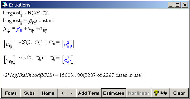
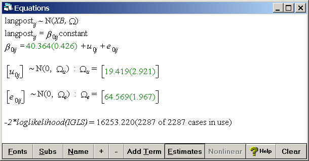
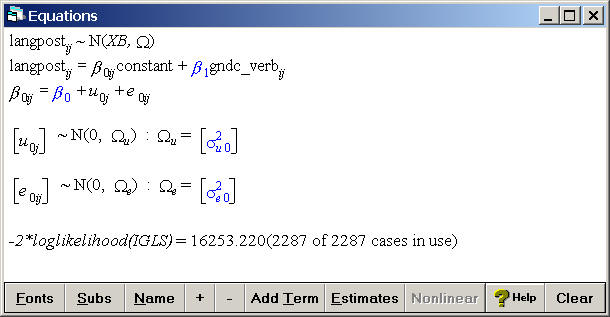
Table 4.1, p. 47.
Estimating the intercept only model using langpost as the dependent variable, schoolnr as level 2 (group level) and pupilnr as level 1 (individual level).
Model
 Equations
  Click on Y
  Choose y: langpost, N levels: 2 - ij, level2(j): schoolnr, and
  level1(i): pupilnr.
   Click on the x0 variable
    Choose the variable constant and select both schoolnr and pupilnr.
     Click on Names, and Estimates at the bottom of the window
      Click on the Start button below the file menu to execute
If the estimates do not appear automatically then click on the estimates button to see the results.
Calculating the grand mean for iq_verb and then creating the variable gndc_verb which is centered around the grand mean.
Basic Statistics
 Averages and Correlations
  Choose iq_verb and click on calculate.
Data Manipulation
  Calculate
    Choose an unused variable and rename it gndc_verb by using ctrl+n
    Enter "gndc_verb" = "iq_verb" - 11.834 and click on calculate.
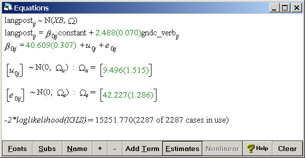
Table 4.2, p. 49.
The model includes only the predictor gndc_verb.
Add Term
 Click on the new term x1
  Choose gndc_verb as a fixed parameter.
Click on the Start button located below the file menu and then click on estimates at the bottom of the equations window to make the estimates appear.
Generate the predicted values from the model in Table 4.2 and storing them in the variable pred.
Model
 Predictions
  in the field called output from prediction to choose an unused variable and rename it
  pred using ctrl+N to bring up the rename window
   Click on Name to see the names of the variables in the model
    Click on constant and gndc_verb which will make all the parameters in the model
    appear in black
     Click on the level 1 error term to make it grey since we do not want to model this error term
      Click on Calc to generate the predicted values and store them in the variable pred
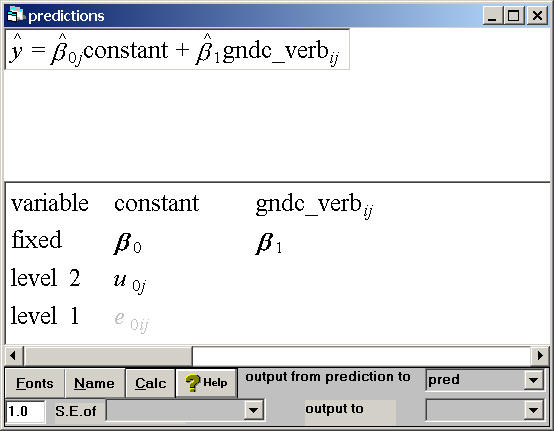
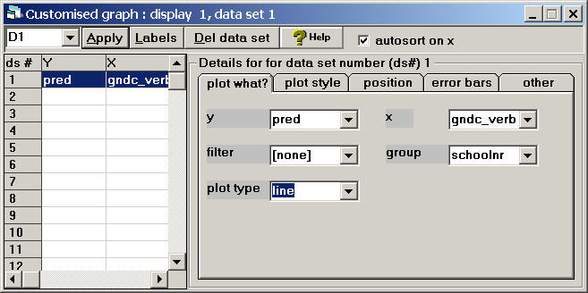
Fig. 4.2, p. 49.
Graphing the regression lines.
Graphs
 Customised Graph(s)
  in the field called y choose pred, for x choose gndc_verb, for group choose schoolnr, and
  for plot type choose line
   Click Apply to generate the graph
Creating the variable grpmc_verb which contains the group means of gndc_verb.
Data Manipulation
 Multilevel Data Manipulation
  in the input column choose gndc_verb, in the output column choose an unused variable and use ctrl+N
  to rename it grpmc_verb then this will be the output variable
   Click Add to action list which will make the input and output choices appear in the action list
   on the right hand side
    Click on Execute
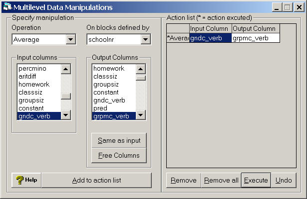
Table 4.4, p. 55
Model including both gndc_verb (within group effect) and grpmc_verb as fixed effects.
Model
 Equations
  Click on Y
  Choose y: langpost, N levels: 2 - ij, level2(j): schoolnr, and
  level1(i): pupilnr.
   Click on the x0 variable
   Choose the variable constant and select both schoolnr and pupilnr.
    Add Term
     Click on the x1 variable
     Choose gndc_verb as a fixed parameter
      Add Term
       Click on the x2 variable
       Choose grpmc_verb as a fixed parameter
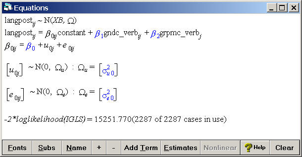
Click on the Start button located below the file menu and then click on estimates at the bottom of the equations window to make the estimates appear.
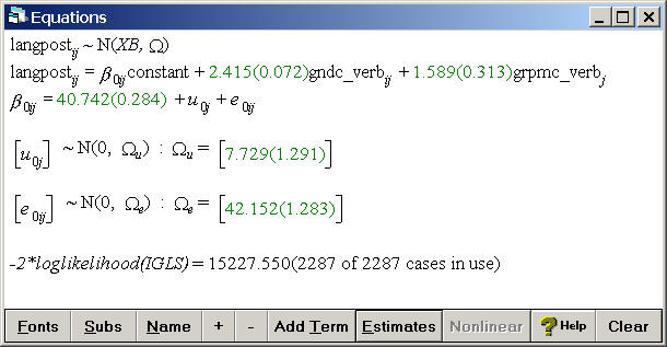
Fig. 4.4, p. 62
The comparative posterior confidence intervals.
Model
 Residuals
  Settings tab
   in the field labeled level choose 2:schoolnr
    in the field labeled SD(comparative) change the value from 1.0 to 1.96
     Click Calc
      Plots tab
       choose residual +/-1.96 sd x rank
        Click Apply
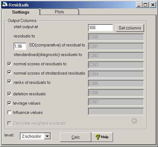
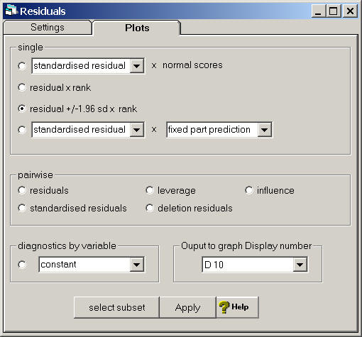
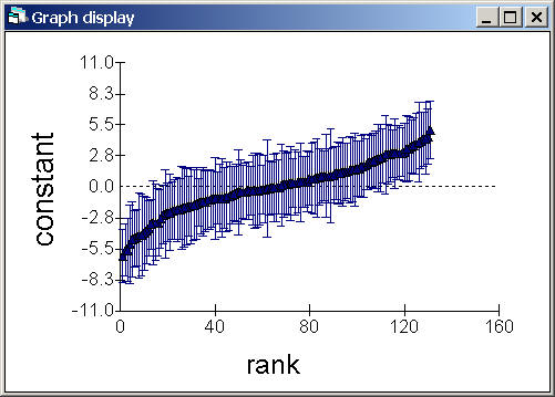
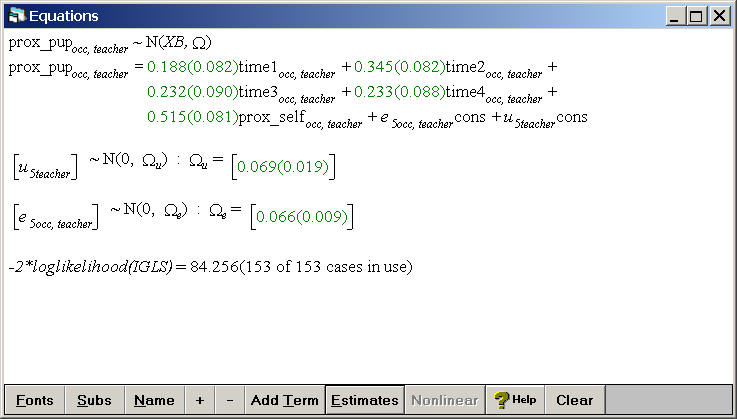
Table 4.5, p. 64 and table 12.6, p. 180.
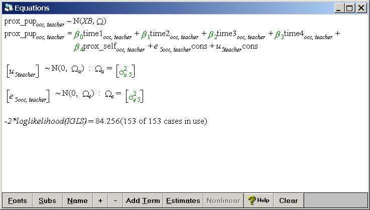
Click on the Start button located below the file menu and then click on estimates at the bottom of the equations window to make the estimates appear.