
Attention
See this FAQ by Bauer that discusses the need to decompose within- and between-group effects when using this approach to ensure valid results (https://dbauer.web.unc.edu/wp-content/uploads/sites/7494/2015/08/Centering-in-111-Mediation.pdf).
FAQ starts here
Version info: Code for this page was tested in SAS 9.3.
Mediator variables are variables that sit between the independent variable and dependent variable and
mediate the effect of the IV on the DV. A model with one mediator is shown in the figure below.
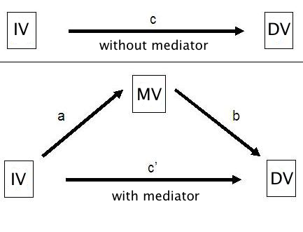
The idea, in mediation analysis, is that some of the effect of the predictor variable, the IV, is transmitted to the DV
through the mediator variable, the MV. And some of the effect of the IV passes directly to the
DV. That portion of of the effect of the IV that passes through the MV is the indirect
effect.
An earlier approach to multilevel mediation suggested by Krull & MacKinnon
(2001) was method 1. This page will demonstrate an alternative approach given in the 2006 paper
by Bauer, Preacher & Gil. This approach combines the dependent variable and the
mediator into a single stacked response variable and runs one mixed model with indicator
variables for the DV and mediator to obtain all of the values needed for the analysis.
We will begin by loading in a synthetic data set and reconfiguring it for our analysis.
All of the variables in this example (id the cluster ID, x the predictor
variable, m the mediator variable, and y the dependent variable)
are at level 1 Here is how the first 16 observations look in the original
dataset. Let’s start by reading in the data and looking at a few descriptive statistics.
filename tmp url 'http://stats.idre.ucla.edu/stat/data/ml_sim.csv';
data ml_sim;
infile tmp dlm=',' firstobs=2;
input id x m y;
fid = _n_;
run;

proc means;
  var id fid x m y;
run;

 The MEANS Procedure

Variable      N            Mean         Std Dev         Minimum         Maximum
-------------------------------------------------------------------------------
id          800      50.5000000      28.8841283       1.0000000     100.0000000
fid         800     400.5000000     231.0844002       1.0000000     800.0000000
x           800      -0.1539876       1.3303736      -4.1514263       3.8696609
m           800      -0.0247739       1.4836143      -6.4783697       5.0124219
y           800      -0.1833981       1.6691804      -8.6000316       5.9190076
-------------------------------------------------------------------------------
There are 100 level-2 units each with eight observations. fid is a row id,
so when the data is not stacked, there is just 1 obsevation for each fid.
Let’s look at the three models of a mediation analysis beginning with the model with just the IV.
proc mixed noclprint;
  class id;
  model y = x / solution;
  random intercept x / subject=id;
run;

 Covariance Parameter Estimates

Cov Parm      Subject    Estimate

Intercept     id           0.7505
x             id           0.2192
Residual                   0.8217

           Fit Statistics
-2 Res Log Likelihood          2435.3
AIC (smaller is better)        2441.3
AICC (smaller is better)       2441.3
BIC (smaller is better)        2449.1


                   Solution for Fixed Effects
                         Standard
Effect       Estimate       Error      DF    t Value    Pr > |t|
Intercept    -0.02737     0.09620      99      -0.28      0.7766
x              0.6907     0.05883      99      11.74
Next, comes the model with the mediator predicted by the IV.
proc mixed noclprint;
  class id;
  model m = x / solution;
  random intercept x / subject=id;
run;

 Covariance Parameter Estimates
Cov Parm      Subject    Estimate
Intercept     id           0.7087
x             id           0.1165
Residual                   0.6451

           Fit Statistics
-2 Res Log Likelihood          2234.6
AIC (smaller is better)        2240.6
AICC (smaller is better)       2240.6
BIC (smaller is better)        2248.4

                   Solution for Fixed Effects
                         Standard
Effect       Estimate       Error      DF    t Value    Pr > |t|
Intercept     0.09519     0.09158      99       1.04      0.3012
x              0.6114     0.04641      99      13.17
Finally, the model with both the IV and mediator predicting the DV.
proc mixed noclprint;
  class id;
  model y = m x / solution;
  random intercept m x / subject=id;
run;

 Covariance Parameter Estimates
Cov Parm      Subject    Estimate
Intercept     id           0.2653
m             id           0.1230
x             id          0.03747
Residual                   0.5070

           Fit Statistics
-2 Res Log Likelihood          2046.8
AIC (smaller is better)        2054.8
AICC (smaller is better)       2054.9
BIC (smaller is better)        2065.3

                   Solution for Fixed Effects
                         Standard
Effect       Estimate       Error      DF    t Value    Pr > |t|
Intercept    -0.09364     0.06251      99      -1.50      0.1373
m              0.6219     0.04721      99      13.17
We see that the IV although still significant has been reduced from .69 to .25.
Now, we need to restructure the data to stack y on m for each row and create
indicator variables for both the mediator and the dependent variables. Here’s how we can do this.
data ml_simlong;
  set ml_sim;
  z = y;
  sy = 1;
  sm = 0;
  dv = 'y';
  output;
  z = m;
  sy = 0;
  sm = 1;
  dv = 'm';
  output;
run;
The new response variable is called z and has y stacked on m.
We named the indicators for the mediator and the DV sm and sy respectively,
to be consistent with Bauer et al (2006). We have also created a new m that
contains the value for the mediator from each of the original observations.
Now we can run our mixed model for multilevel mediation using proc mixed.
Notice that because we include the sm and sy indicators
in the model that we need to use the noint option for the fixed effects
(it is not automatically included for random effects, so there is no need to supress it).
In addition to the random effects, we use a repeated subcommand to model the heterogeneity in
residual variances for y and m (which are now stacked and just in the variable z.
proc mixed data=ml_simlong noclprint covtest;
  class id dv;
  model z = sm sm * x sy sy * m sy * x /noint solution covb;
  random sm sm * x sy sy * m sy * x / subject=id type=un;
  repeated / group=dv subject=id;
run;

The Mixed Procedure

                  Model Information

Data Set                     WORK.ML_SIMLONG
Dependent Variable           z
Covariance Structures        Unstructured, Variance
                             Components
Subject Effects              id, id
Group Effect                 dv
Estimation Method            REML
Residual Variance Method     None
Fixed Effects SE Method      Model-Based
Degrees of Freedom Method    Containment


            Dimensions

Covariance Parameters            17
Columns in X                      5
Columns in Z Per Subject          5
Subjects                        100
Max Obs Per Subject              16


          Number of Observations

Number of Observations Read            1600
Number of Observations Used            1600
Number of Observations Not Used           0


                     Iteration History

Iteration    Evaluations    -2 Res Log Like       Criterion

        0              1      5018.02760634
        1              4      4324.76342851     50.66699378
        2              3      4303.83578771     29.81384239
        3              2      4284.51183182     26.06489084
        4              1      4262.57000555      0.02711155
        5              2      4253.92727615      0.00276758
        6              2      4252.35296469      0.00012231
        7              1      4252.26931686      0.00000042
        8              1      4252.26903780      0.00000000


                   Convergence criteria met.
                      Covariance Parameter Estimates

                                             Standard         Z
Cov Parm     Subject    Group    Estimate       Error     Value        Pr Z

UN(1,1)      id                    0.6794      0.1132      6.00      0.09896     0.02282      4.34       ChiSq

    16        765.76           |t|

sm         0.09321     0.08943      99       1.04      0.2998
sm*x        0.6119     0.04650      99      13.16      0.6106     0.04554      99      13.41      0.2208     0.03725      99       5.93      0.002162    0.000127    0.000985    -0.00020
   3    sy        0.000576    0.000127    0.003839    -0.00011    -0.00006
   4    sy*m      0.000093    0.000985    -0.00011    0.002074    -0.00048
   5    x*sy      -0.00006    -0.00020    -0.00006    -0.00048    0.001387


       Type 3 Tests of Fixed Effects

           Num     Den
Effect      DF      DF    F Value    Pr > F

sm           1      99       1.09    0.2998
sm*x         1      99     173.17
We now have access to all of the information needed to compute the average indirect
effect and average total effect and their standard errors using the equations
given in Bauer, et. al. (2006).
ind = ab + sigma_{a_{j}b_{j}} quad (EQ:A11)
] [
Var(ind) = b^{2}sigma^{2}_{hat{a}} + a^{2}sigma^{2}_{hat{b}} +
sigma^{2}_{hat{a}}sigma^{2}_{hat{b}} + 2absigma_{hat{a},hat{b}} +
(sigma_{hat{a},hat{b}})^2 + sigma^{2}_{hat{sigma}_{a_{j},b_{j}}} quad (EQ:A14)
]
average total effect
[tot = ab + sigma_{a_{j}b_{j}} + c’ quad (EQ:A15)
] [
Var(ind) = b^{2}sigma^{2}_{hat{a}} + a^{2}sigma^{2}_{hat{b}} +
2absigma_{hat{a},hat{b}} + 2bsigma_{hat{a},hat{c}’} + 2asigma_{hat{b},hat{c}’} +
sigma^{2}_{hat{sigma}_{a_{j},b_{j}}} + sigma^{2}_{hat{c}’} +
sigma^{2}_{hat{a}}sigma^{2}_{hat{b}} + (sigma_{hat{a},hat{b}})^2 quad (EQ:A18)
]
These formulae involve the fixed effects estimates, their variances and covariances,
and variances and covariances from the random effects. The values used are highlighted in
yellow in the SAS output above.
a = 0.6119
b = 0.6106
c’ = 0.2208
sigma_{a_{j}b_{j}} = 0.09896
sigma^{2}_{hat{a}} = 0.002162
sigma^{2}_{hat{b}} = 0.002074
sigma_{hat{a},hat{b}} = 0.000985
sigma_{hat{a},hat{c}’} = -0.00020
sigma_{hat{b},hat{c}’} = -0.00048
sigma^{2}_{hat{c}’} = 0.001387
sigma^{2}_{hat{sigma}_{a_{j},b_{j}}} = 0.02282^{2}
]
To calculate this, you just need a calculator. A simple way in SAS is using SAS’ matrix language,
in PROC IML, which essentially allows us to just declare the constants and write out the
formulae.
proc iml;
  a = 0.6119;
  b = 0.6106;
  rcov_ab = 0.09896;
  cprime = 0.2208;
  Va = 0.002162;
  Vb = 0.002074;
  Vcprime = 0.001387;
  cov_ab = 0.000985;
  cov_ac = -0.00020;
  cov_bc = -0.00048;
  Vcov_ab = 0.022822**2;

  ind_eff = a*b + rcov_ab;
  V_ind_eff = a**2*Vb + b**2*Va + Va*Vb + 2*a*b*cov_ab + cov_ab**2 + Vcov_ab;
  test_ind = ind_eff/V_ind_eff**.5;
  tot_eff = ind_eff + cprime;
  V_tot_eff = b**2*Va + a**2*Vb + Va*Vb + 2*a*b*cov_ab + cov_ab**2 + Vcprime + 2*b*cov_ac + 2*a*cov_bc + Vcov_ab;
  test_tot = tot_eff/V_tot_eff**.5;

  print ind_eff; /* indirect effect */
  print V_ind_eff; /* variance of indirect effect */
  print test_ind; /* significance test of indirect effect, test against standard normal */
  print tot_eff; /* total effect */
  print V_tot_eff; /* variance of total effect */
  print test_tot; /* significance test of total effect, test against standard normal */
quit;

 ind_eff
0.4725861

V_ind_eff
 0.002845

 test_ind
8.8601944

 tot_eff
0.6933861

V_tot_eff
0.0034003

 test_tot
11.890965
We get the indirect effect, the variance of the indirect effect, and a test value
(the effect divided by its standard error), which we could calculate a p-value for by
comparing it against the standard normal distribution. For anything greater than
roughly 1.96 will be statistically significant at p = .05.
See also
If you do not want to calculate this all out by hand, you can go to
Daniel Bauer’s website,
where he has posted a PDF of the publication this page is based on
as well as his own examples, and a SAS macro to calculate and test
the indirect effects.
References
- Bauer, D. J., Preacher, K. J. & Gil, K. M. (2006) Conceptualizing and testing random indirect
effects and moderated mediation in multilevel models: New procedures and recommendations.
Psychological Methods, 11(2), 142-163. - Krull, J. L. & MacKinnon, D. P. (2001) Multilevel modeling of individual and group level
mediated effects. Multivariate Behavioral Research, 36(2), 249-277.