
Let’s use an example data set called crf24.
data crf24;
  input y a b;
  cards;
3 1 1
4 1 2
7 1 3
7 1 4
1 2 1
2 2 2
5 2 3
10 2 4
6 1 1
5 1 2
8 1 3
8 1 4
2 2 1
3 2 2
6 2 3
10 2 4
3 1 1
4 1 2
7 1 3
9 1 4
2 2 1
4 2 2
5 2 3
9 2 4
3 1 1
3 1 2
6 1 3
8 1 4
2 2 1
3 2 2
6 2 3
11 2 4
;
run;
These are data from a 2 by 4 factorial
design. The variable y is the dependent variable. The
variable a is an independent variable with two levels while b is
an independent variable with four levels. Let’s look at a table of cell
means and standard deviations.
proc means data=crf24 mean std;
  class a b;
  var y;
run;
The MEANS Procedure Analysis Variable : y N a b Obs Mean Std Dev ------------------------------------------------------------------- 1 1 4 3.7500000 1.5000000 2 4 4.0000000 0.8164966 3 4 7.0000000 0.8164966 4 4 8.0000000 0.8164966 2 1 4 1.7500000 0.5000000 2 4 3.0000000 0.8164966 3 4 5.5000000 0.5773503 4 4 10.0000000 0.8164966 -------------------------------------------------------------------
Now let’s run the ANOVA. We will get the
predicted values, call them yhat, and save them in a temporary data
file called crf24p. We will use these predicted values in a
moment when we create a graph of the cell means.
proc glm data=crf24;
  class a b;
  model y = a b a*b;
  output out=crf24p p=yhat;
run;
quit;
The GLM Procedure Class Level Information Class Levels Values a 2 1 2 b 4 1 2 3 4 Number of observations 32 Dependent Variable: y Sum of Source DF Squares Mean Square F Value Pr > F Model 7 217.0000000 31.0000000 40.22 <.0001 Error 24 18.5000000 0.7708333 Corrected Total 31 235.5000000 R-Square Coeff Var Root MSE y Mean 0.921444 16.33435 0.877971 5.375000 Source DF Type I SS Mean Square F Value Pr > F a 1 3.1250000 3.1250000 4.05 0.0554 b 3 194.5000000 64.8333333 84.11 <.0001 a*b 3 19.3750000 6.4583333 8.38 0.0006 Source DF Type III SS Mean Square F Value Pr > F a 1 3.1250000 3.1250000 4.05 0.0554 b 3 194.5000000 64.8333333 84.11 <.0001 a*b 3 19.3750000 6.4583333 8.38 0.0006
We see that in addition to a significant main effect
for b there is a significant a*b interaction effect.
Before we do any of the tests of simple main effects, let’s graph the cell
means to get an idea of what the interaction looks like. The following
sequence of commands will produce a graph of the cell means. Note that
in order to make a graph with the predicted values for each level of a,
a data step is necessary to separate the predicted values into two new
variables, which we call yhat1 and yhat2. We then plot
both yhat1 and yhat2 against b and overlay the two
graphs.
data crf24q;
   set crf24p;
   if a = 1 then yhat1 = yhat;
   if a = 2 then yhat2 = yhat;
run;

proc sort data = crf24q;
  by b;
run;

symbol1 i=join;
symbol2 i = join line = 3;
proc gplot data=crf24q;
  plot yhat1*b = 1 yhat2*b = 2/overlay;
run;
quit;
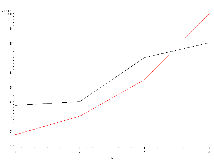
The interaction is clearly shown where the two lines
cross over between levels b3 and b4. We will now do a test
of simple main effects looking at differences in a at each level of b.
proc glm data=crf24;
  class a b;
  model y = a b a*b;
  lsmeans a*b / slice = b;
run;
quit;
The GLM Procedure Class Level Information Class Levels Values a 2 1 2 b 4 1 2 3 4 Number of observations 32 Dependent Variable: y Sum of Source DF Squares Mean Square F Value Pr > F Model 7 217.0000000 31.0000000 40.22 <.0001 Error 24 18.5000000 0.7708333 Corrected Total 31 235.5000000 R-Square Coeff Var Root MSE y Mean 0.921444 16.33435 0.877971 5.375000 Source DF Type I SS Mean Square F Value Pr > F a 1 3.1250000 3.1250000 4.05 0.0554 b 3 194.5000000 64.8333333 84.11 <.0001 a*b 3 19.3750000 6.4583333 8.38 0.0006 Source DF Type III SS Mean Square F Value Pr > F a 1 3.1250000 3.1250000 4.05 0.0554 b 3 194.5000000 64.8333333 84.11 <.0001 a*b 3 19.3750000 6.4583333 8.38 0.0006 Least Squares Means a b y LSMEAN 1 1 3.7500000 1 2 4.0000000 1 3 7.0000000 1 4 8.0000000 2 1 1.7500000 2 2 3.0000000 2 3 5.5000000 2 4 10.0000000 a*b Effect Sliced by b for y Sum of b DF Squares Mean Square F Value Pr > F 1 1 8.000000 8.000000 10.38 0.0036 2 1 2.000000 2.000000 2.59 0.1203 3 1 4.500000 4.500000 5.84 0.0237 4 1 8.000000 8.000000 10.38 0.0036
There is a statistically significant effect
for each level of b except for level 2. However, one may want to
consider the effect of performing multiple tests on the family-wise error rate
and perhaps adjust the critical alpha level accordingly. Using a
Bonferonni correction, the critical alpha level would be .0125 instead of .05
(.05/4). Using the Bonferonni criteria, comparisons one and four would
be considered statistically significant.
Note:
Statisticians do not universally approve of the use of tests of simple
main effects. In particular, there are concerns over the conceptual error
rate. Tests of simple main effects are one tool that can be useful in
interpreting interactions. In general, the results of tests of simple
main effects should be considered suggestive and not definitive.