
Let’s read in an example dataset, crf24, adapted from Kirk (1968,
First Edition).
get file 'c:https://stats.idre.ucla.edu/wp-content/uploads/2016/02/crf24.sav'.
These data are from a 2×4 factorial design. The variable y is the dependent variable. The variable a is an independent variable with two levels, while b is an independent variable with four levels. Let’s look at a table of cell means and standard deviations.
means table = y by a by b.
Case Processing Summary
Cases
Included
Excluded
Total
N
Percent
N
Percent
N
Percent
Y * A * B
32
100.0%
0
.0%
32
100.0%
Report
Y
A
B
Mean
N
Std. Deviation
1
1
3.75
4
1.500
2
4.00
4
.816
3
7.00
4
.816
4
8.00
4
.816
Total
5.69
16
2.120
2
1
1.75
4
.500
2
3.00
4
.816
3
5.50
4
.577
4
10.00
4
.816
Total
5.06
16
3.316
Total
1
2.75
8
1.488
2
3.50
8
.926
3
6.25
8
1.035
4
9.00
8
1.309
Total
5.38
32
2.756
Now let’s run the ANOVA.
glm y by a b.
Between-Subjects Factors
N
A
1
16
2
16
B
1
8
2
8
3
8
4
8
Tests of Between-Subjects Effects
Dependent Variable: Y
Source
Type III Sum of Squares
df
Mean Square
F
Sig.
Corrected Model
217.000(a)
7
31.000
40.216
.000
Intercept
924.500
1
924.500
1199.351
.000
A
3.125
1
3.125
4.054
.055
B
194.500
3
64.833
84.108
.000
A * B
19.375
3
6.458
8.378
.001
Error
18.500
24
.771
Total
1160.000
32
Corrected Total
235.500
31
a R Squared = .921 (Adjusted R Squared = .899)
We see that in addition to a significant main effect for b there is a significant a*b interaction effect. Before we do any of the tests of simple main effects, let’s graph the cell means to get an idea of what the interaction looks like.
You can include a /plot subcommand with the glm command to get a
plot of the cell means.
glm y by a b
 /plot = profile(b*a).
<output omitted>
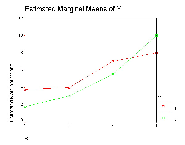
The interaction is clearly shown where the two lines cross over between levels b3 and b4. We will now do a test of simple main effects looking at differences in a at each level of b. This is done by including a /emmeans subcommand with the glm
command.
glm y by a b
 /emmeans = tables(a*b)compare(a).
Between-Subjects Factors
N
A
1
16
2
16
B
1
8
2
8
3
8
4
8
Tests of Between-Subjects Effects
Dependent Variable: Y
Source
Type III Sum of Squares
df
Mean Square
F
Sig.
Corrected Model
217.000(a)
7
31.000
40.216
.000
Intercept
924.500
1
924.500
1199.351
.000
A
3.125
1
3.125
4.054
.055
B
194.500
3
64.833
84.108
.000
A * B
19.375
3
6.458
8.378
.001
Error
18.500
24
.771
Total
1160.000
32
Corrected Total
235.500
31
a R Squared = .921 (Adjusted R Squared = .899)
Estimates
Dependent Variable: Y
Mean
Std. Error
95% Confidence Interval
A
B
Lower Bound
Upper Bound
1
1
3.750
.439
2.844
4.656
2
4.000
.439
3.094
4.906
3
7.000
.439
6.094
7.906
4
8.000
.439
7.094
8.906
2
1
1.750
.439
.844
2.656
2
3.000
.439
2.094
3.906
3
5.500
.439
4.594
6.406
4
10.000
.439
9.094
10.906
Pairwise Comparisons
Dependent Variable: Y
Mean Difference (I-J)
Std. Error
Sig.(a)
95% Confidence Interval for Difference(a)
B
(I) A
(J) A
Lower Bound
Upper Bound
1
1
2
2.000(*)
.621
.004
.719
3.281
2
1
-2.000(*)
.621
.004
-3.281
-.719
2
1
2
1.000
.621
.120
-.281
2.281
2
1
-1.000
.621
.120
-2.281
.281
3
1
2
1.500(*)
.621
.024
.219
2.781
2
1
-1.500(*)
.621
.024
-2.781
-.219
4
1
2
-2.000(*)
.621
.004
-3.281
-.719
2
1
2.000(*)
.621
.004
.719
3.281
Based on estimated marginal means
* The mean difference is significant at the .050 level.
a Adjustment for multiple comparisons: Least Significant Difference (equivalent to no adjustments).
Univariate Tests
Dependent Variable: Y
B
Sum of Squares
df
Mean Square
F
Sig.
1
Contrast
8.000
1
8.000
10.378
.004
Error
18.500
24
.771
2
Contrast
2.000
1
2.000
2.595
.120
Error
18.500
24
.771
3
Contrast
4.500
1
4.500
5.838
.024
Error
18.500
24
.771
4
Contrast
8.000
1
8.000
10.378
.004
Error
18.500
24
.771
Each F tests the simple effects of A within each level combination of the other effects shown. These tests are based on the linearly independent pairwise comparisons among the estimated marginal means.
Note:
Statisticians do not universally approve of the use of tests of simple
main effects. In particular, there are concerns over the conceptual error
rate. Tests of simple main effects are one tool that can be useful in
interpreting interactions. Caution should be exercised in interpreting
the results of analyses of simple main effects. In general, the results of tests of simple
main effects should be considered suggestive and not definitive.
You can get more information on this topic by visiting: